Background

The initial inspiration for this work was the Data for Democracy NYC Accessibility project (Project GitHub Repo), which focused on exploring the lack of ADA-accessible stations in the New York City subway system. For those that are unfamiliar, ADA-accessible subway stations are those that comply with the Americans with Disabilities Act of 1990. Among other requirements, they must be designed such that an individual using a wheelchair or other mobility device can get from street level to the turnstiles and onto the train.

New York City’s subway system is one of the busiest in the world, with a weekday average ridership of 5.6 million as of 2017, but it is also the least accessible transit system in the United States. While the ADA focuses on individuals with disabilities, an ADA-compliant system is friendlier to all, from parents with young children and strollers to the elderly. An excuse for the state of things might be the age of the system since the NYC subway is among one of the older ones in the country. However, other mass transit systems that opened around the same time, such as the ones in Boston and Chicago, have a far higher percentage of compliant stations.

The accessibility problem is a symptom of the larger set of issues that have plagued the city’s transit system for years now. The subways are slow and overcrowded, the trains manage to be on time only 65% of the time (although this has increased to 70% as of December 2018), and the whole of the MTA, the body responsible for the subway along with other transit systems in the area, has been financially mismanaged to the brink of ruin. As an example of said mismanagement, the MTA invested in its bus system and Access-a-Ride, a door-to-door service, in an effort to increase accessibility instead of converting subway stations. But, not only is a system of buses not comparable in terms of speed and service quality to the subway, this decision wound up costing the MTA more money than it would have to retrofit elevators in subway stations. As of today, plans are underway to fix the centuries-old signal systems, increase train speeds, and to install elevators at existing stations to make them accessible. But given the previous track record, there is cause for concern about whether the NYC subway system can turn things around, or maybe Elon Musk will save the day in the end.

Project goals

Project focus

I had been curious about geospatial analysis for a while, and this project was a great excuse to learn more. However, this project also turned out to require quite a lot of data cleaning, especially for the Subway Entrances and Exits dataset.

In the end, the main data science-related skills that are the focus of this project are:

• Data exploration and cleaning - I had severely underestimated how messy and out of date the NYC Subway Entrances and Exits dataset was. It needed quite a lot of manual curation to reach an analysis-ready state.
• Geospatial analysis in R - mapping, spatial joins, converting non-spatial data into a spatial format, and more, mainly with the help of the sf package. As an aside, this DataCamp course on the sf package, led by Zev Ross, was immensely helpful in this regard.

Packages

Packages used:

• tidyverse - omnibus package for data import, wrangling, and cleaning (never leave home without it)
• sf - for geospatial data analysis
• ggthemes - ggplot2 theme and palette add-on
• mapview - easy to use package for creating quick interactive maps

library(tidyverse)
library(sf)
library(ggthemes)
library(mapview)
# minimal theme for nice plots throughout the project
theme_set(theme_minimal())

Data

Shapefiles, imported using the st_read function from the sf package:

• nyc.census.map: Shapefile of NYC 2010 census tract boundaries
• nyc.neigh.map: Shapefile of NYC neighborhoods

Datasets, in .csv format:

• subway.ent.exit: The Subway Entrances and Exits dataset that provides information about what train routes stop at each station, whether the stations are ADA-accessible or not, as well as the station latitude and longitude coordinates, but in a non-spatial format with no coordinate reference system (CRS).
  
• subway.by.line: In NYC, the subway routes are grouped into “trunk lines”, typically based on their route through Manhattan, and the grouping can indicate which trains share many of the same station stops. Each trunk line also has its own distinct assigned color that appears on the subway route symbols. This dataset lists the routes that belong to each trunk line and their respective color codes.
• num.stat.by.rt.wiki: This is a list of the number of station stops by route, according to their Wikipedia pages. The data will be used later to clean the subway entrances and exits dataset. NYC subway service changes over the course of the day and the weekend, with some lines switching from express to local or going out of service altogether. In this analysis, I will be focusing on the weekday rush-hour service because, in theory, that is when the most number of people should be using the subway.

### shapefiles ###
nyc.census.map <- st_read("./data/r_geospatial_project/nyct2010_18a/nyct2010.shp")

Reading layer `nyct2010' from data source `C:\Users\Dasha\Documents\GitHub\personal_website\content\post\data\r_geospatial_project\nyct2010_18a\nyct2010.shp' using driver `ESRI Shapefile'
Simple feature collection with 2166 features and 11 fields
geometry type:  MULTIPOLYGON
dimension:      XY
bbox:           xmin: 913175.1 ymin: 120121.9 xmax: 1067383 ymax: 272844.3
epsg (SRID):    NA
proj4string:    +proj=lcc +lat_1=40.66666666666666 +lat_2=41.03333333333333 +lat_0=40.16666666666666 +lon_0=-74 +x_0=300000 +y_0=0 +datum=NAD83 +units=us-ft +no_defs

nyc.neigh.map <- st_read("./data/r_geospatial_project/nynta_18d/nynta.shp")

Reading layer `nynta' from data source `C:\Users\Dasha\Documents\GitHub\personal_website\content\post\data\r_geospatial_project\nynta_18d\nynta.shp' using driver `ESRI Shapefile'
Simple feature collection with 195 features and 7 fields
geometry type:  MULTIPOLYGON
dimension:      XY
bbox:           xmin: 913175.1 ymin: 120121.9 xmax: 1067383 ymax: 272844.3
epsg (SRID):    NA
proj4string:    +proj=lcc +lat_1=40.66666666666666 +lat_2=41.03333333333333 +lat_0=40.16666666666666 +lon_0=-74 +x_0=300000 +y_0=0 +datum=NAD83 +units=us-ft +no_defs

### subway info ###
subway.ent.exit <- read_csv("./data/r_geospatial_project/NYC_Transit_Subway_Entrance_And_Exit_Data.csv")
subway.by.line <- read_csv("./data/r_geospatial_project/nyc_subway_stations_grouped.csv")
num.stat.by.rt.wiki <- read_csv("./data/r_geospatial_project/nyc_subway_num_stat_by_line.csv")

Data sources:

• NYC Census Map shapefile: NYC Department of City Planning Open Data Website
• NYC Neighborhood Tabulation Areas Map shapefile: NYC Department of City Planning Open Data Website
• Subway Entrances and Exits: Open Data NY
• Subway by Line Info: Copied from the NYC Subway Wikipedia Page, Nomenclature section
• Number of Subway Stations by Route: Manually collected from each individual subway route page, such as this page for the E subway service

Data preview

The NYC census tract and neighborhood sf files can be visualized in many ways, including with the ggplot2 package and the plot function. Here, ggplot is used to layer the census tracts in blue and the neighborhood boundaries in orange to demonstrate the difference, for those not familiar with the city.

# nyc census tracts map in blue
nyc.census.map %>% 
  ggplot() +
  geom_sf(color = "#1F77B4") +
  # nyc neighborhoods outlines overlaid in orange
  geom_sf(data = nyc.neigh.map, color = "#FF7F0E", size = 1, fill = NA) +
  ggtitle("NYC census tracts and neighborhoods") +
  xlab("Longitude") +
  ylab("Latitude")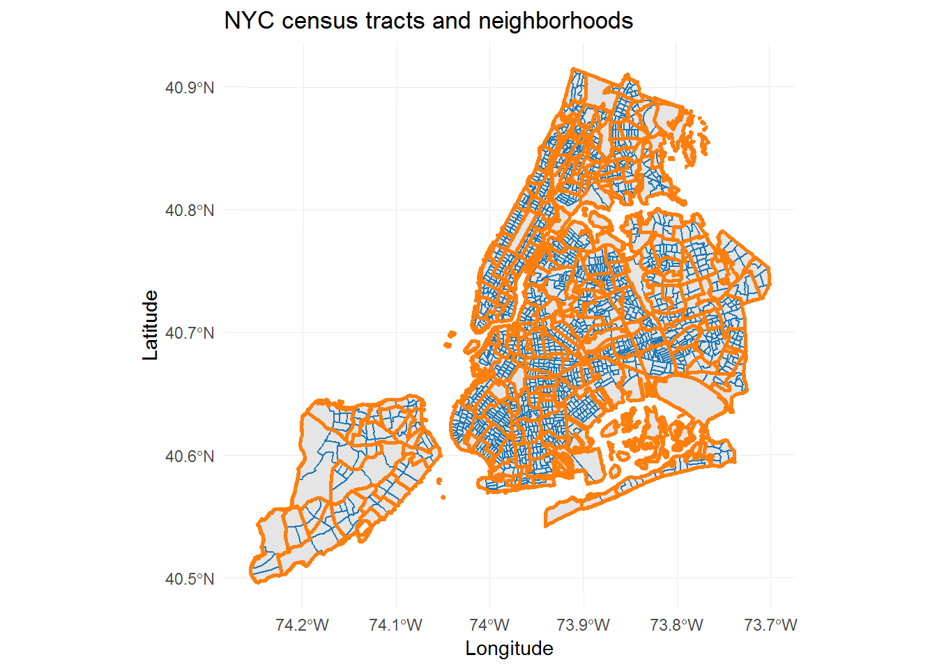

Most neighborhoods contain multiple census tracts, except for parks and airports, and each census tract is part of only one neighborhood. Both shapefiles include Staten Island, for which there is no data in the subway entrances/exits dataset, and therefore it will be removed from further consideration.

On top of being spatial objects, a handy feature of the sf format is that these objects are also data frames and can be treated as such for filtering, joining, and other data wrangling manipulations.

summary(nyc.census.map)

    CTLabel     BoroCode          BoroName       CT2010       BoroCT2010  
 138    :   5   1:288    Bronx        :339   003300 :   5   1000100:   1  
 151    :   5   2:339    Brooklyn     :760   003900 :   5   1000201:   1  
 247    :   5   3:760    Manhattan    :288   007500 :   5   1000202:   1  
 251    :   5   4:668    Queens       :668   007700 :   5   1000500:   1  
 279    :   5   5:111    Staten Island:111   013800 :   5   1000600:   1  
 33     :   5                                015100 :   5   1000700:   1  
 (Other):2136                                (Other):2136   (Other):2160  
 CDEligibil    NTACode                    NTAName          PUMA     
 E:1002     BK50   :  34   Canarsie           :  34   4009   :  83  
 I:1164     BK31   :  28   Bay Ridge          :  28   4112   :  80  
            BK88   :  28   Borough Park       :  28   4105   :  68  
            BK58   :  27   Crown Heights North:  27   4103   :  65  
            BK61   :  27   East New York      :  27   4110   :  65  
            BK82   :  27   Flatlands          :  27   4101   :  59  
            (Other):1995   (Other)            :1995   (Other):1746  
   Shape_Leng         Shape_Area                 geometry   
 Min.   :   168.5   Min.   :      582   MULTIPOLYGON :2166  
 1st Qu.:  5622.6   1st Qu.:  1683579   epsg:NA      :   0  
 Median :  6496.8   Median :  1987942   +proj=lcc ...:   0  
 Mean   :  8726.0   Mean   :  3891726                       
 3rd Qu.:  8734.1   3rd Qu.:  3189156                       
 Max.   :186126.0   Max.   :196238540                       
                                                            

For example, as demonstrated above, the nyc.census.map object includes the tract codes, the city borough name that the census tract belongs to, as well as the spatial geometry.

As for the other datasets, the Subway Entrances and Exits dataset contains the most useful and relevant information for this project. However, it will require considerable transformation to get it into a usable format, and will have to be given a CRS and converted into a spatial sf object at some point.

# subway entrances/exit data:
glimpse(subway.ent.exit)

Observations: 1,868
Variables: 30
$ Division             <chr> "BMT", "BMT", "BMT", "BMT", "BMT", "BMT",...
$ Line                 <chr> "4 Avenue", "4 Avenue", "4 Avenue", "4 Av...
$ `Station Name`       <chr> "25th St", "25th St", "36th St", "36th St...
$ `Station Latitude`   <dbl> 40.66040, 40.66040, 40.65514, 40.65514, 4...
$ `Station Longitude`  <dbl> -73.99809, -73.99809, -74.00355, -74.0035...
$ Route1               <chr> "R", "R", "N", "N", "N", "R", "R", "R", "...
$ Route2               <chr> NA, NA, "R", "R", "R", NA, NA, NA, NA, NA...
$ Route3               <chr> NA, NA, NA, NA, NA, NA, NA, NA, NA, NA, N...
$ Route4               <chr> NA, NA, NA, NA, NA, NA, NA, NA, NA, NA, N...
$ Route5               <chr> NA, NA, NA, NA, NA, NA, NA, NA, NA, NA, N...
$ Route6               <chr> NA, NA, NA, NA, NA, NA, NA, NA, NA, NA, N...
$ Route7               <chr> NA, NA, NA, NA, NA, NA, NA, NA, NA, NA, N...
$ Route8               <dbl> NA, NA, NA, NA, NA, NA, NA, NA, NA, NA, N...
$ Route9               <dbl> NA, NA, NA, NA, NA, NA, NA, NA, NA, NA, N...
$ Route10              <dbl> NA, NA, NA, NA, NA, NA, NA, NA, NA, NA, N...
$ Route11              <dbl> NA, NA, NA, NA, NA, NA, NA, NA, NA, NA, N...
$ `Entrance Type`      <chr> "Stair", "Stair", "Stair", "Stair", "Stai...
$ Entry                <chr> "YES", "YES", "YES", "YES", "YES", "YES",...
$ `Exit Only`          <chr> NA, NA, NA, NA, NA, NA, NA, NA, NA, NA, N...
$ Vending              <chr> "YES", "YES", "YES", "YES", "YES", "YES",...
$ Staffing             <chr> "FULL", "NONE", "FULL", "FULL", "FULL", "...
$ `Staff Hours`        <chr> NA, NA, NA, NA, NA, NA, NA, NA, NA, NA, N...
$ ADA                  <lgl> FALSE, FALSE, FALSE, FALSE, FALSE, FALSE,...
$ `ADA Notes`          <chr> NA, NA, NA, NA, NA, NA, NA, NA, NA, NA, N...
$ `Free Crossover`     <lgl> FALSE, FALSE, TRUE, TRUE, TRUE, TRUE, TRU...
$ `North South Street` <chr> "4th Ave", "4th Ave", "4th Ave", "4th Ave...
$ `East West Street`   <chr> "25th St", "25th St", "36th St", "36th St...
$ Corner               <chr> "SE", "SW", "NW", "NE", "NW", "NE", "NW",...
$ `Entrance Latitude`  <dbl> 40.66032, 40.66049, 40.65449, 40.65436, 4...
$ `Entrance Longitude` <dbl> -73.99795, -73.99822, -74.00450, -74.0041...

# subway route groupings and color codes:
glimpse(subway.by.line)

Observations: 10
Variables: 4
$ `Primary Trunk line` <chr> "IND Eighth Avenue Line", "IND Sixth Aven...
$ Color                <chr> "Vivid blue", "Bright orange", "Lime gree...
$ Hexadecimal          <chr> "#2850ad", "#ff6319", "#6cbe45", "#a7a9ac...
$ Lines                <chr> "A_C_E", "B_D_F_M", "G", "L", "J_Z", "N_Q...

# number of station stops by route:
glimpse(num.stat.by.rt.wiki)

Observations: 25
Variables: 4
$ route_name        <chr> "A", "C", "E", "B", "D", "F", "M", "G", "L",...
$ num_stations_norm <dbl> 44, 40, 22, 27, 36, 45, 36, 21, 24, 30, 21, ...
$ late_night        <dbl> 66, NA, 32, NA, 41, NA, 8, NA, NA, NA, NA, 4...
$ limited           <dbl> NA, NA, 19, 37, NA, NA, 13, NA, NA, 20, NA, ...

Let’s start with the following:

• Remove Staten Island from the maps since the subway datasets do not include Staten Island transit routes
• subway.ent.exit: The entrances and exits dataset is very messy. It needs cleaning, and the route columns need to be reorganized into a tidy format. Will also need to evaluate how useful some of the other columns that relate to the specific entrances and exits might be.
• subway.by.line: Needs to be tidied, with each subway route on its own row.
• num.stat.by.rt.wiki: Is fine as is.

First cleaning

To start off with the maps, Staten Island will be filtered out and the column names will be converted to lowercase for later convenience.

nyc.census.4boro <- nyc.census.map %>%  
  filter(BoroName != "Staten Island") %>% 
  `colnames<-`(str_to_lower(colnames(nyc.census.map)))
nyc.neigh.4boro <- nyc.neigh.map %>% 
  filter(BoroName != "Staten Island") %>% 
  `colnames<-`(str_to_lower(colnames(nyc.neigh.map)))
# new column names:
colnames(nyc.census.4boro)

 [1] "ctlabel"    "borocode"   "boroname"   "ct2010"     "boroct2010"
 [6] "cdeligibil" "ntacode"    "ntaname"    "puma"       "shape_leng"
[11] "shape_area" "geometry"  

colnames(nyc.neigh.4boro)

[1] "borocode"   "boroname"   "countyfips" "ntacode"    "ntaname"   
[6] "shape_leng" "shape_area" "geometry"  

# new map (neighborhoods only): 
ggplot(nyc.neigh.4boro) +
  geom_sf(aes(fill = boroname), color = "white") +
  ggtitle("NYC neighborhoods\n(No Staten Island)") +
  xlab("Longitude") +
  ylab("Latitude") +
  # tableau palette from ggthemes, ordered to match later plots
  scale_fill_manual(values = c("#76B7B2", "#F28E2B","#4E79A7", "#E15759"), name = "Borough") +
  # prevent overlapping text on x-axis:
  theme(axis.text.x = element_text(angle = 45, hjust = 1))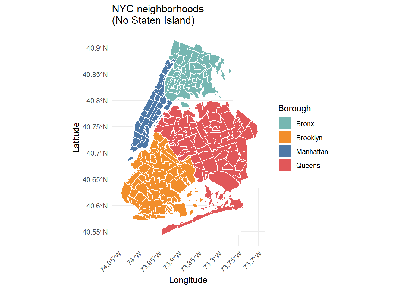

The column names of the other two subway datasets that needed cleaning will be modified by converting them to lowercase and by replacing the empty spaces to make them easier to work with.

colnames(subway.ent.exit) <- colnames(subway.ent.exit) %>% 
  str_to_lower() %>% 
  str_replace_all(" ", "_")
colnames(subway.by.line) <- colnames(subway.by.line) %>% 
  str_to_lower() %>% 
  str_replace_all(" ", "_")
# result:
colnames(subway.ent.exit)

 [1] "division"           "line"               "station_name"      
 [4] "station_latitude"   "station_longitude"  "route1"            
 [7] "route2"             "route3"             "route4"            
[10] "route5"             "route6"             "route7"            
[13] "route8"             "route9"             "route10"           
[16] "route11"            "entrance_type"      "entry"             
[19] "exit_only"          "vending"            "staffing"          
[22] "staff_hours"        "ada"                "ada_notes"         
[25] "free_crossover"     "north_south_street" "east_west_street"  
[28] "corner"             "entrance_latitude"  "entrance_longitude"

colnames(subway.by.line)

[1] "primary_trunk_line" "color"              "hexadecimal"       
[4] "lines"             

Much better!

Next, the lines column in the subway.by.line dataset needs to be separated and wrangled so that each subway line is its own row.

sub.line.tidy <- subway.by.line %>% 
  # converts lines into a list conlumn
  transform(lines = strsplit(lines, "_")) %>%
  # unnests the list column and converts each into a separate row
  unnest(lines) %>% 
  # rename to match other df
  rename(route_name = lines)
# result:
head(sub.line.tidy)

      primary_trunk_line         color hexadecimal route_name
1 IND Eighth Avenue Line    Vivid blue     #2850ad          A
2 IND Eighth Avenue Line    Vivid blue     #2850ad          C
3 IND Eighth Avenue Line    Vivid blue     #2850ad          E
4  IND Sixth Avenue Line Bright orange     #ff6319          B
5  IND Sixth Avenue Line Bright orange     #ff6319          D
6  IND Sixth Avenue Line Bright orange     #ff6319          F

Now that that dataset is clean, it is possible to check the route names against the entrances/exits data in order to determine if there is anything odd.

subway.ent.exit %>% 
  # gather the unique route names across all of the route columns in the subway ent/exit dataset:
  select(route1:route11) %>% 
  gather("route_num", "route_name") %>% 
  filter(!(is.na(route_name))) %>% 
  select(-route_num) %>% 
  distinct() %>% 
  # any route names in the ent/exit df that are not in the official subway route list on the wiki?
  anti_join(sub.line.tidy, by = "route_name")

# A tibble: 4 x 1
  route_name
  <chr>     
1 GS        
2 FS        
3 e         
4 H         

Yes, it looks like there are four routes in the subway entrance/exit data that are not on the Wikipedia route list. However, the e is simply a typo that should be capitalized to E, which is a real route, and the three routes GS, FS, and H all fall under the umbrella of S in the wiki route list. The three are separate, relatively short routes that are designated as shuttles (hence the “S” name). GS is the 42nd St shuttle in Manhattan that only stops in Times Square and Grand Central. FS is the Franklin Avenue shuttle that operates between Franklin Ave and Prospect Park in Brooklyn. Lastly, H is the Rockaways shuttle in Queens. The discrepancy in route names is something to keep in mind for later, but not an error that needs to be fixed.

It is time to switch focus to the dataset that is the core of this project: the subway entrances and exits data. According to Wikipedia, the official city count is that there are 472 individual subway stations in NYC, or 424 if connected stations are counted as a single station. I expect that the raw dataset will be off to some extent because I’ve already discovered that it has not even been updated with the opening of the Second Avenue Subway in January of 2017 and the changes to Q train service, which added 3 stations in Manhattan. So how many subway stations are there in the data right now?

# number of unique subway station names:
length(unique(subway.ent.exit$station_name))

[1] 356

That is far too few stations, but it’s not a surprise given that station names are often reused in NYC. For example, there are five “23rd Street” stations in Manhattan and one in Queens. Therefore, the station_name column alone cannot be used as a unique key for the stations in this dataset.

What are some other options? The subway by line dataset had special codes and names to refer to the trunk line, such as IRT and BMT, which seem to match the division and line columns in the entrances/exits data. I suspect that the division, line, and station_name columns will give the unique identifier for each station. But how many distinct combinations of those three columns are there?

# what the columns look like:
subway.ent.exit %>% 
  select(division:station_name) %>% 
  distinct() %>% 
  head()

# A tibble: 6 x 3
  division line     station_name
  <chr>    <chr>    <chr>       
1 BMT      4 Avenue 25th St     
2 BMT      4 Avenue 36th St     
3 BMT      4 Avenue 45th St     
4 BMT      4 Avenue 53rd St     
5 BMT      4 Avenue 59th St     
6 BMT      4 Avenue 77th St     

# count unique division, line, and station_name column combinations:
subway.ent.exit %>% 
  select(division:station_name) %>% 
  distinct() %>% 
  nrow()

[1] 465

There are 465 such combinations, which is close to the expected 472 number. Adding in 3 missing new Q train stations brings the number up, but there may be more stations missing from the dataset than I thought.

As an aside, how many station name, latitude, and longitude combinations are there?

subway.ent.exit %>% 
  select(station_name, station_latitude:station_longitude) %>% 
  distinct() %>% 
  nrow()

[1] 473

The count of the unique station name, latitude, and longitude combinations is more than there are stations, or even division/line/station name combinations, which suggests that the geographical coordinates are not the best choices for a unique key. On further exploration, it turned out that some stations had multiple sets of coordinates. This may be related to the entrances and exits locations, or possibly due to physical connections between stations.

Based on the above, the next steps for the cleanup of the subway entrance/exit dataset are:

• Create a unique station name column by combining the division, line, and station name which will be treated as the unique key column from now on
• Fix the capitalization typo in the route columns
• To fix the issue of the same station having multiple geographical coordinates, take the average of the latitude and longitude for each station and then use these values as the station location coordinates

sub.ent.w.key <- subway.ent.exit %>% 
  # convert the 3 columns to lowercase
  mutate_at(vars(division:station_name), str_to_lower) %>% 
  # create a unique key for each station
  unite("stat_name", division:station_name, sep = "_") %>% 
  # capitalize all of the route names (to fix the e issue)
  mutate_at(vars(route1:route11), str_to_upper) 
# result:
head(sub.ent.w.key %>% select(stat_name:station_longitude))

# A tibble: 6 x 3
  stat_name            station_latitude station_longitude
  <chr>                           <dbl>             <dbl>
1 bmt_4 avenue_25th st             40.7             -74.0
2 bmt_4 avenue_25th st             40.7             -74.0
3 bmt_4 avenue_36th st             40.7             -74.0
4 bmt_4 avenue_36th st             40.7             -74.0
5 bmt_4 avenue_36th st             40.7             -74.0
6 bmt_4 avenue_45th st             40.6             -74.0

# coordinates fix:
sub.ent.w.key <- sub.ent.w.key %>% 
  # get rid of original coordinates:
  select(-c(station_latitude:station_longitude)) %>% 
  distinct() %>% 
  # join onto average coordinates:
  left_join(
    # get the average lat and average long for each station:
    sub.ent.w.key %>% 
      select(stat_name:station_longitude) %>% 
      distinct() %>% 
      group_by(stat_name) %>% 
      summarize(
        avg_stat_lat = mean(station_latitude),
        avg_stat_long = mean(station_longitude)
        ),
    by = "stat_name"
    )
# resulting number of stations:
length(unique(sub.ent.w.key$stat_name))

[1] 465

# number of unique geographical coordinates:
sub.ent.w.key %>% 
  select(avg_stat_lat:avg_stat_long) %>% 
  distinct() %>% 
  nrow()

[1] 462

It looks like some of the subway stations have the same geographical coordinates, which will need to be explored further later on. But first, let’s look at the station entrance/exit-related columns in the dataset and determine what, if anything, might be useful for the purposes of this project.

Entrance analysis

Apart from the subway station location information, the entrances and exits dataset provides information on, well, the entrances and exits. Included are the entrance/exit geographical coordinates, entry type, as well as an ADA rating, in a TRUE or FALSE format. Do these columns provide any extra insights and are they worth carrying along?

First, how many of each entrance type are there and what is the relationship between the entrance type and the ADA-accessibility rating of the station?

# count each entrance type:
table(sub.ent.w.key$entrance_type)

     Door  Easement  Elevator Escalator      Ramp     Stair   Walkway 
       81        91        49        28         3      1614         1 

# count ada ratings:
table(sub.ent.w.key$ada)

FALSE  TRUE 
 1400   467 

Stairs are by far the most common entrance/exit type, which is something new learned, but the ADA count by itself doesn’t say much. I’m curious if the ADA rating is on a per-station or per-entrance basis?

sub.ent.w.key %>% 
  group_by(stat_name) %>% 
  summarize(
    # count total number of entrances per station:
    num_entry = n(),
    # ada is TRUE/FALSE - can sum to get number of ada = TRUE per station:
    num_ada = sum(ada),
    # % ada out of total num of entrances, per station:
    percent_ada = num_ada * 100 / num_entry
    ) %>% 
  {table(.$percent_ada)}

  0 100 
381  84 

The result is that the stations are either 0% ADA or 100% ADA, which indicates that the ADA TRUE/FALSE rating is given to the entire station and not to the particular entrance/exit. This suddenly makes the entrances/exits columns a lot less interesting to me, and I will remove them from consideration after a few more plots.

But first, let’s ask what the most common entrance/exit types for ADA-accessible and not accessible stations are?

sub.ent.w.key %>% 
  group_by(entrance_type, ada) %>% 
  count() %>% 
  ggplot(aes(entrance_type, n, fill = ada)) +
  geom_bar(stat = "identity", position = "dodge") +
  xlab("Entrance/Exit type") +
  ylab("Count") +
  scale_fill_tableau(name = "ADA Status") +
  ggtitle("Entrance/Exit count by ADA rating and type")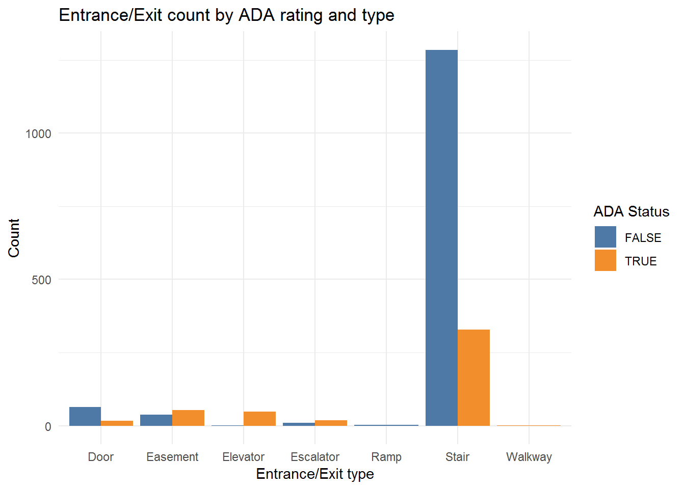

Stairs by far are the most common form of access, and in general, stations that have stair entrances are more often ADA == FALSE than not, but the size of the stairs bars dominates the plot. Let’s switch perspectives with position = "fill" in the geom_bar call.

sub.ent.w.key %>% 
  group_by(entrance_type, ada) %>% 
  count() %>% 
  ggplot(aes(entrance_type, n, fill = ada)) +
  geom_bar(stat = "identity", position = "fill") +
  xlab("Entrance/Exit type") +
  ylab("Proportion") +
  scale_fill_tableau(name = "ADA Status") +
  ggtitle("Entrance/Exit count by ADA rating and type\n(Bars fill position)")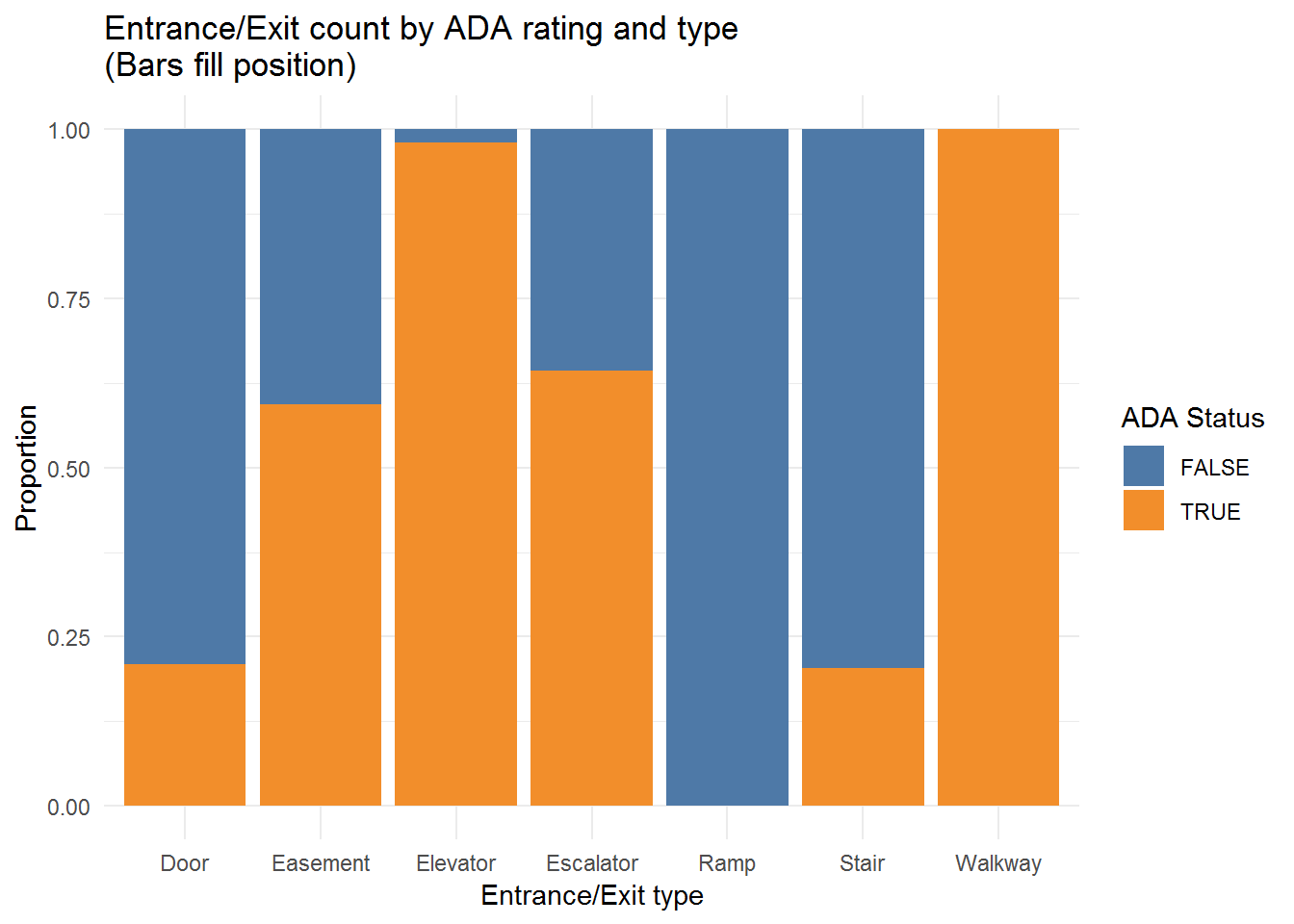

This alternative view shows that “Elevator” entrances tend to be linked to ADA-accessible stations. I tried to search, but I’m not sure what an “Easement” entrance may be. It seems to indicate a private access point, perhaps meant to be used for utility work. Typical accessible routes are elevators and escalators, which can explain why the elevator and escalator ADA == TRUE bars are high relative to other entrance types, although I believe an elevator is required for a station to be rated fully ADA-accessible.

Removing entrance info and more tidying

Next, the entrance/exit columns will be removed because they are no longer useful to me, and the route columns will be wrangled into a tidy format. In order to replicate the maps in the official report, the route information would also not be needed and could be dropped at this point. However, I’m interested in how many stations are located within particular geographical areas, and so the route columns will be carried along. The plan, for now, is that I intend to count each individual train route that stops at a station. For example, if three train routes, such as the 4, 5, and 6 trains, all stop at one station, I would like to be able to count each of those, for a total of three, because the more trains stop in a given area, the more “accessible” or reachable by subway that area is and I want to account for that.

With these goals in mind, let’s get to tidying.

sub.ent.sml <- sub.ent.w.key %>% 
  # select relevant columns, discard all others from this point on
  select(stat_name, avg_stat_lat:avg_stat_long, route1:route11, ada, ada_notes) %>% 
  distinct() %>% 
  # reformat the route columns into a long format
  gather("route_num", "route_name", route1:route11) %>% 
  # get rid of the many NAs in the route column that were there due to the formatting
  filter(!is.na(route_name)) %>% 
  select(-route_num) %>% 
  distinct()
# new format dimensions:
dim(sub.ent.sml)

[1] 985   6

head(sub.ent.sml)

# A tibble: 6 x 6
  stat_name           avg_stat_lat avg_stat_long ada   ada_notes route_name
  <chr>                      <dbl>         <dbl> <lgl> <chr>     <chr>     
1 bmt_4 avenue_25th ~         40.7         -74.0 FALSE <NA>      R         
2 bmt_4 avenue_36th ~         40.7         -74.0 FALSE <NA>      N         
3 bmt_4 avenue_45th ~         40.6         -74.0 FALSE <NA>      R         
4 bmt_4 avenue_53rd ~         40.6         -74.0 FALSE <NA>      R         
5 bmt_4 avenue_59th ~         40.6         -74.0 FALSE <NA>      N         
6 bmt_4 avenue_77th ~         40.6         -74.0 FALSE <NA>      R         

# number of unique stations and train route combinations:
sub.ent.sml %>% 
  select(stat_name, route_name) %>% 
  distinct() %>% 
  nrow()

[1] 980

# missing values check:
sapply(sub.ent.sml, anyNA)

    stat_name  avg_stat_lat avg_stat_long           ada     ada_notes 
        FALSE         FALSE         FALSE         FALSE          TRUE 
   route_name 
        FALSE 

At least in terms of formatting, the new subway station data frame is much neater, with each route now in its own row instead of in columns. Along with the ADA rating and station location, I’ve also carried on the ada_notes column which is not NA for only a few stations and should be easier to explore now that the dataset of interest is much smaller.

Trouble ahead

Let’s take a look at the ada_notes column and the stations for which it is not NA.

sub.ent.sml %>% 
  select(stat_name, ada, ada_notes) %>% 
  distinct() %>% 
  filter(!(is.na(ada_notes))) %>% 
  arrange(stat_name, ada)

# A tibble: 13 x 3
   stat_name                                  ada   ada_notes        
   <chr>                                      <lgl> <chr>            
 1 bmt_broadway_49th st                       TRUE  Northbound Only  
 2 bmt_broadway_times square-42nd st          TRUE  Shuttle not ADA  
 3 bmt_broadway_union square                  TRUE  Lex not ADA      
 4 bmt_canarsie_union square                  TRUE  Lex not ADA      
 5 ind_8 avenue_50th st                       TRUE  Southbound Only  
 6 ind_8 avenue_world trade center            TRUE  Construction     
 7 ind_archer av_sutphin blvd-archer av - jfk TRUE  Check            
 8 ind_concourse_kingsbridge rd               FALSE in planning      
 9 ind_queens boulevard_forest hills-71st av  FALSE in planning      
10 irt_lexington_23rd st                      FALSE In Planning      
11 irt_lexington_brooklyn bridge-city hall    TRUE  J Z not ADA      
12 irt_lexington_canal st                     TRUE  Bway Nass not ADA
13 irt_pelham_hunts point av                  FALSE in planning      

Some observations and next steps:

• It looks like ADA changes were under construction or in planning at the time that this data was compiled. The associated stations need to be checked, and the ADA-status changed from FALSE to TRUE if changes were completed.
• A few of the stations are ADA-accessible in only one direction (northbound or southbound). I decided to allow ADA == TRUE for the entire station if it was ADA-accessible in at least one direction because it would be challenging to count a station as “half-accessible” to account for this.
• Even though my earlier analysis suggested that the stations were either completely ADA-accessible or not at all, the notes make it clear that some stations are not fully accessible for all train routes. The Union Square station is rated as ADA-accessible for the L, N, Q, R, and W trains, but not for the Lexington Ave 4, 5, and 6 trains, even though ADA == TRUE for the entire station (see: bmt_broadway_union square and bmt_canarsie_union square with the note Lex not ADA). This might be a consequence of the original data formatting, and, because for me it is essential to get the station stops count right, I will need to explore this issue further and correct the ADA rating where appropriate.
• Some stations seem to be listed twice because different trunk line trains stop there. For example, again, Union Square, which is considered one station, is listed as bmt_broadway_union square for the N/Q/R/W trunk line and bmt_canarsie_union square for the L trunk line. These duplicates will need to be removed for an accurate count of train routes down the line.

After exploring the dataset more, I stumbled onto more problems. Most worrying for my purposes was that it turned out that train route names are repeated for each connected station. Case in point, there is a World Trade Center stop where only the E train should stop. But some subway stations are connected underground by tunnels so that one can transfer from one station to another, and the World Trade Center stop is one such station. If I filter for this station only, where only the E should stop, instead there are 5 trains listed.

sub.ent.sml %>% 
  filter(stat_name == "ind_8 avenue_world trade center")

# A tibble: 5 x 6
  stat_name          avg_stat_lat avg_stat_long ada   ada_notes  route_name
  <chr>                     <dbl>         <dbl> <lgl> <chr>      <chr>     
1 ind_8 avenue_worl~         40.7         -74.0 TRUE  Construct~ A         
2 ind_8 avenue_worl~         40.7         -74.0 TRUE  Construct~ C         
3 ind_8 avenue_worl~         40.7         -74.0 TRUE  Construct~ E         
4 ind_8 avenue_worl~         40.7         -74.0 TRUE  Construct~ 2         
5 ind_8 avenue_worl~         40.7         -74.0 TRUE  Construct~ 3         

This is because the World Trade Center stop is connected to the Park Place, where the 2 and 3 trains stop, and Chambers St, where the A and C stop.

If I select for the Park Place station information, it turns out that all of the trains are repeated at this station as well (and the same is true for Chambers St).

sub.ent.sml %>% 
  filter(stat_name == "irt_clark_park place")

# A tibble: 6 x 6
  stat_name           avg_stat_lat avg_stat_long ada   ada_notes route_name
  <chr>                      <dbl>         <dbl> <lgl> <chr>     <chr>     
1 irt_clark_park pla~         40.7         -74.0 FALSE <NA>      A         
2 irt_clark_park pla~         40.7         -74.0 FALSE <NA>      C         
3 irt_clark_park pla~         40.7         -74.0 FALSE <NA>      E         
4 irt_clark_park pla~         40.7         -74.0 FALSE <NA>      1         
5 irt_clark_park pla~         40.7         -74.0 FALSE <NA>      2         
6 irt_clark_park pla~         40.7         -74.0 FALSE <NA>      3         

Thankfully, the ADA rating is separate from the World Trade Center station and is correctly marked as FALSE at Park Place. However, the issue is that all of the trains are also listed as stopping at this station, as well as the 1 train even though the 1 route should not follow the 2 and 3 in this part of Manhattan.

I initially thought about using the division and line columns that went into creating the unique station names to filter the extra trains somehow. Based on the data I got from Wikipedia, the associated “line” names with the IND division, for example, should only be:

sub.line.tidy %>% 
  filter(str_detect(primary_trunk_line, "IND")) %>% 
  select(primary_trunk_line) %>% 
  distinct()

      primary_trunk_line
1 IND Eighth Avenue Line
2  IND Sixth Avenue Line
3     IND Crosstown Line

However, the line names for the same division in the subway entrances/exit data are far more varied.

sub.ent.sml %>%
  select(stat_name) %>% 
  distinct() %>% 
  # select only the IND division subway station stops
  filter(str_detect(stat_name, "ind")) %>% 
  # separate out the different name parts again
  separate(stat_name, into = c("division", "line", "station_name"), sep = "_") %>% 
  {table(.$line)}

        6 avenue      63rd street         8 avenue        archer av 
              20                3               31                3 
       concourse        crosstown           culver           fulton 
              11               12               10               15 
         liberty queens boulevard         rockaway 
               7               24               14 

Yes, the 8th Ave, 6th Ave, and Crosstown lines are there (although in a different format), but there are several other line names, likely because the modern subway lines were built up over time and many of the current routes are combinations of the old ones. This suggests that I cannot reliably use the line information, and maybe even the division codes to filter the subway station and train route combinations.

On further exploration, it also seems that the dataset was far more out of date than expected. For example, the G train route is missing station stops between Smith 9th St and Church Ave, where its service was extended along the F route in 2009. The problem is best seen overlaid on a map of the city. I had mentioned earlier that the subway entrances/exits dataset, while it did include geospatial coordinates, did not come with a coordinate reference system (CRS). A CRS is important because it defines the units of the spatial object. Trying to work with two objects with different CRS would be like comparing distances measured in inches to kilometers, it wouldn’t make sense. Based on some research, it seems that the subway location data should have “+init=epsg:4326” as its CRS. For now, I won’t worry about turning the subway data to a spatial object and converting its CRS to match the NYC shapefiles. Instead, I can transform the city shapefiles and take advantage of the ggplot2 system of layers to superimpose the subway data over a map.

# transform the neighborhood map crs to march the subway entrance/exit data:
nyc.map.4boro.stat.crs <- st_transform(nyc.neigh.4boro, crs = "+init=epsg:4326")
nyc.map.4boro.stat.crs %>% 
  ggplot() +
  # plot the neighborhoods
  geom_sf(fill = NA) +
  # plot the F and G subway lines
  geom_point(
    data = sub.ent.sml %>% 
      filter(route_name == "F" | route_name == "G"),
    aes(avg_stat_long, avg_stat_lat, color = route_name),
    size = 2, 
    alpha = 0.8
    ) +
  xlab("Longitude") +
  ylab("Latitude") +
  scale_color_tableau(name = "Route") +
  ggtitle("G and F train routes (Outdated)") +
  theme(axis.text.x = element_text(angle = 45, hjust = 1))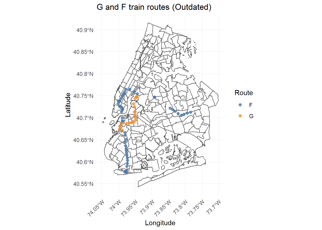

In its current state, the dataset has G service terminating at the Smith-Ninth Streets stop. Luckily, in this case, the missing stations could just be added in by attaching a part of the F train route to the G train.

# get the slice of F train stations that are missing from the G route: 
sub.ent.sml %>% 
  filter(route_name == "F") %>% 
  arrange(avg_stat_lat) %>% 
  filter(avg_stat_lat > 40.62976 & avg_stat_lat < 40.68030)

# A tibble: 8 x 6
  stat_name           avg_stat_lat avg_stat_long ada   ada_notes route_name
  <chr>                      <dbl>         <dbl> <lgl> <chr>     <chr>     
1 ind_culver_ditmas ~         40.6         -74.0 FALSE <NA>      F         
2 ind_6 avenue_churc~         40.6         -74.0 TRUE  <NA>      F         
3 ind_6 avenue_fort ~         40.7         -74.0 FALSE <NA>      F         
4 ind_6 avenue_prosp~         40.7         -74.0 FALSE <NA>      F         
5 ind_6 avenue_7th av         40.7         -74.0 FALSE <NA>      F         
6 ind_6 avenue_4th av         40.7         -74.0 FALSE <NA>      F         
7 bmt_4 avenue_9th st         40.7         -74.0 FALSE <NA>      F         
8 ind_6 avenue_smith~         40.7         -74.0 FALSE <NA>      F         

# extra station for the connected 4 Av-9 St stations (the stop after Smith-Ninth Streets):
# G train is considered IND - grab that 4th ave station
sub.ent.sml <- sub.ent.sml %>% 
  # create a copy of the F train station stops for this section of track
  bind_rows(
    sub.ent.sml %>% 
      filter(route_name == "F") %>% 
      arrange(avg_stat_lat) %>% 
      filter(avg_stat_lat > 40.63612 & avg_stat_lat < 40.67358 & str_detect(stat_name, "ind")) %>% 
      # change the route name for this section 
      mutate(route_name = "G")
    )
# example at Church Ave
sub.ent.sml %>%
  filter(stat_name == "ind_6 avenue_church av")

# A tibble: 2 x 6
  stat_name           avg_stat_lat avg_stat_long ada   ada_notes route_name
  <chr>                      <dbl>         <dbl> <lgl> <chr>     <chr>     
1 ind_6 avenue_churc~         40.6         -74.0 TRUE  <NA>      F         
2 ind_6 avenue_churc~         40.6         -74.0 TRUE  <NA>      G         

# now both the F and G are at Church Ave
# Updated G train route:
nyc.map.4boro.stat.crs %>% 
  ggplot() +
  geom_sf(fill = NA) +
  geom_point(
    data = sub.ent.sml %>% 
      filter(route_name == "F" | route_name == "G"),
    aes(avg_stat_long, avg_stat_lat, color = route_name),
    size = 2, 
    alpha = 0.8
    ) +
  xlab("Longitude") +
  ylab("Latitude") +
  scale_color_tableau(name = "Route") +
  ggtitle("G and F train routes (Updated)") +
  theme(axis.text.x = element_text(angle = 45, hjust = 1))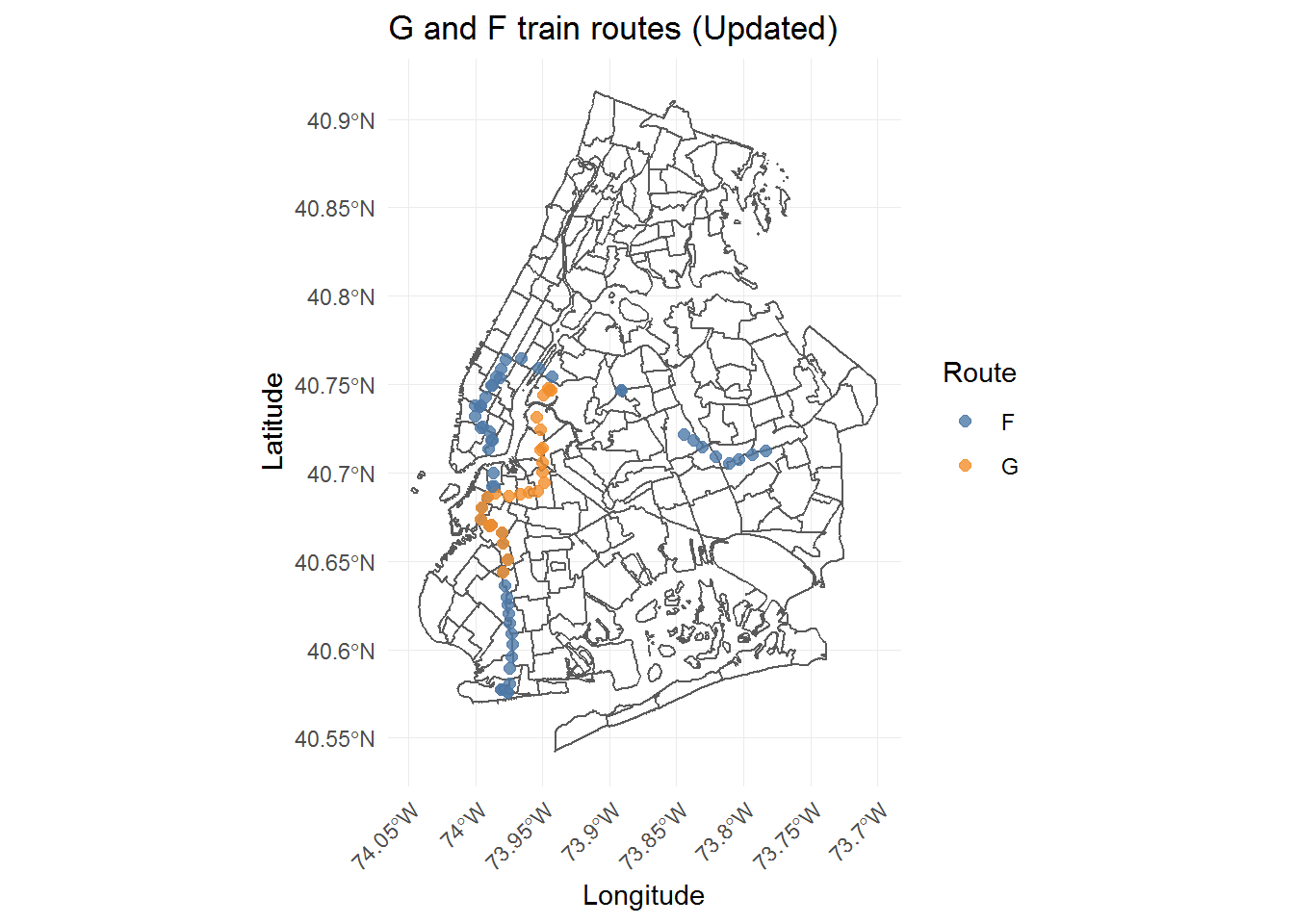

The updated route start and end stations are correct, but now there are more stations than expected based on the Wikipedia station count.

# expected number:
num.stat.by.rt.wiki %>% 
  filter(route_name == "G")

# A tibble: 1 x 4
  route_name num_stations_norm late_night limited
  <chr>                  <dbl>      <dbl>   <dbl>
1 G                         21         NA      NA

# new number of G train stations:
sub.ent.sml %>%
  filter(route_name == "G") %>% 
  nrow()

[1] 25

At this point, I’m starting to think that I’ll need to check through the station and train associations manually, but first I will go back to the ada_notes issues, deal with those, and drop the column before moving on.

ADA fixes and hitting a wall

Changes to make based on the ada_notes:

• ind_8 avenue_50th st / TRUE / Southbound Only: Leave as ada = TRUE (no changes)
• ind_8 avenue_world trade center / TRUE / Construction: ada = TRUE for E only
• ind_archer av_sutphin blvd-archer av - jfk / TRUE / Check: ada = TRUE according to wikipedia page (no change)
• bmt_broadway_49th st / TRUE / Northbound Only: Leave as ada = TRUE (no change)
• bmt_broadway_times square-42nd st / TRUE / Shuttle not ADA: set S to ada = FALSE
• bmt_broadway_union square / TRUE / Lex not ADA: set 4/5/6 to ada = FALSE
  
• bmt_canarsie_union square / TRUE / Lex not ADA: same as above
  
• ind_concourse_kingsbridge rd / FALSE / in planning: switch to TRUE because it has been completed
  
• irt_lexington_23rd st / FALSE In Planning: switch to TRUE because it has been completed
• irt_lexington_brooklyn bridge-city hall / TRUE / J Z not ADA: set J/Z to ada = FALSE
• irt_lexington_canal st / TRUE / Bway Nass not ADA: Only set 6 ada = TRUE
• irt_pelham_hunts point av / FALSE / in planning: complete, set ada = TRUE
  
• ind_queens boulevard_forest hills-71st av / FALSE / in planning: complete, set ada = TRUE

Another small fix is that I noticed is that there are two redundant routes, GS and S, that refer to the same thing: the grand central shuttle between times square and grand central. The “S” route will be filtered out and the ADA rating for the GS route will be changed to FALSE because it is not ADA-accessible at both Times Square and Grand Central.

I chose to keep each change as a separate mutate call to keep track of the changes, although it is messy.

sub.ent.ada.updt <- sub.ent.sml %>% 
  # change world trade center station ada
  mutate(ada = ifelse((stat_name == "ind_8 avenue_world trade center" & route_name != "E"), FALSE, ada)) %>% 
  # change times square shuttle ada, filter out extra "S" route
  filter(route_name != "S") %>% 
  mutate(ada = ifelse(route_name == "GS", FALSE, ada)) %>% 
  # change 4/5/6 at union square to ada = FALSE
  mutate(ada = ifelse(
    ((stat_name == "bmt_broadway_union square" | stat_name == "bmt_canarsie_union square") & (route_name == "4" | route_name == "5" | route_name == "6")),
    FALSE, ada
    )) %>% 
  # change kingsbridge rd ada = TRUE
  mutate(ada = ifelse(stat_name == "ind_concourse_kingsbridge rd", TRUE, ada)) %>% 
  # change Lex / 23rd St stop to TRUE
  mutate(ada = ifelse(stat_name == "irt_lexington_23rd st", TRUE, ada)) %>% 
  # change J/Z at Brooklyn Bridge / City Hall to ada = FALSE
  mutate(ada = ifelse(
    (stat_name == "irt_lexington_brooklyn bridge-city hall" & (route_name == "J" | route_name == "Z")),
    FALSE, ada
    )) %>% 
  # change irt_lexington_canal st to ada = TRUE for 6 train only
  mutate(ada = ifelse(
    (stat_name == "irt_lexington_canal st" & route_name != "6"), FALSE, ada
    )) %>% 
  # change rt 6 hunts point av to ada = TRUE
  mutate(ada = ifelse(stat_name == "irt_pelham_hunts point av", TRUE, ada)) %>% 
  # convert the forst hills / 71st ave station to ada = TRUE for all lines
  mutate(ada = ifelse(stat_name == "ind_queens boulevard_forest hills-71st av", TRUE, ada)) %>% 
  # can get rid of the ada_notes column now
  select(-ada_notes) %>% 
  distinct()
# original length:
dim(sub.ent.sml)

[1] 990   6

# updated version slightly smaller:
dim(sub.ent.ada.updt)

[1] 982   5

# original S route:
sub.ent.sml %>% 
  filter(route_name == "S")

# A tibble: 3 x 6
  stat_name         avg_stat_lat avg_stat_long ada   ada_notes   route_name
  <chr>                    <dbl>         <dbl> <lgl> <chr>       <chr>     
1 ind_8 avenue_42n~         40.8         -74.0 TRUE  <NA>        S         
2 bmt_broadway_tim~         40.8         -74.0 TRUE  Shuttle no~ S         
3 irt_broadway-7th~         40.8         -74.0 TRUE  <NA>        S         

# Now S route is gone:
sub.ent.ada.updt %>% 
  filter(route_name == "S")

# A tibble: 0 x 5
# ... with 5 variables: stat_name <chr>, avg_stat_lat <dbl>,
#   avg_stat_long <dbl>, ada <lgl>, route_name <chr>

# GS still there, but has duplicate stops:
sub.ent.ada.updt %>% 
  filter(route_name == "GS")

# A tibble: 4 x 5
  stat_name                     avg_stat_lat avg_stat_long ada   route_name
  <chr>                                <dbl>         <dbl> <lgl> <chr>     
1 irt_42nd st shuttle_grand ce~         40.8         -74.0 FALSE GS        
2 irt_flushing_grand central-4~         40.8         -74.0 FALSE GS        
3 irt_lexington_grand central-~         40.8         -74.0 FALSE GS        
4 irt_42nd st shuttle_times sq~         40.8         -74.0 FALSE GS        

Got rid of a few rows by eliminating the redundant S route, and removed the ada_notes column.

Now back to the earlier issue of trains being assigned to subway stations that they do not stop at and all the previous problems brought up earlier.

How does the number of stations in the subway entrances/exit dataset per route compare to the expected number (according to Wikipedia)?

stat.count.join <- sub.ent.ada.updt %>% 
  group_by(route_name) %>% 
  count() %>% 
  full_join(num.stat.by.rt.wiki, by = "route_name") %>% 
  # W exits in the wiki df, but not in the sub ent/exit df
  filter(route_name != "W")
stat.count.join %>% 
  ggplot(aes(num_stations_norm, n)) +
  # equality line for refence:
  geom_abline(intercept = 0, slope = 1, size = 1, linetype = "dashed") +
  geom_point(size = 2, alpha = 0.8) +
  xlab("Expected station count by route") +
  ylab("Actual station count by route")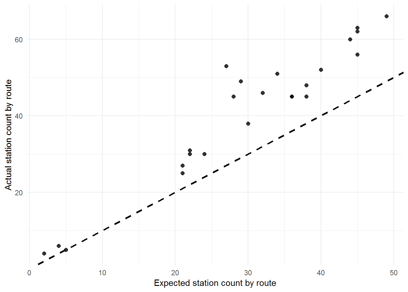

stat.count.join %>% 
  filter(num_stations_norm == n)

# A tibble: 1 x 5
# Groups:   route_name [1]
  route_name     n num_stations_norm late_night limited
  <chr>      <int>             <dbl>      <dbl>   <dbl>
1 H              5                 5         NA      NA

Nearly all of the trains, except for the H shuttle route, have more subway stations assigned to them than expected. The extra stations are not accounted for by different service patterns (such as local late-night service). Based on what was seen earlier from the data, the likely sources of the issues are:

• Stations are duplicated if different division and trunk line trains service it, and all of the routes that stop at the station are listed for each instance of that station in the dataset.
• The dataset is outdated - no updates were made as service changed over the years or when construction projects were completed.
• Separate stations connected by underground tunnels were listed as one station, with all routes servicing both stations (e.g., the E train and the World Trade Center, Park Place, and Chambers St stations situation).

At this point, the options, as I saw them, were:

Solution 1: Import a dataset form the NYC Open Data website with updated subway route data and try to merge the ADA data with the new station information.

Problems with Solution 1: Subway station names repeat, which means that a lot of manual data cleaning and validation would still be required to make sure the stations merged correctly. Also, if the subway route information is out of date, likely the ADA status of stations would also need updating (this assumption turns out to be correct in the end).

Solution 2: Manually go through each route using official NYC subway station listings to make sure that the information is accurate and to remove station duplicates.

Problems with Solution 2: Will require a lot of tedious manual work, and there’s always the risk of making mistakes. Will have to manually add-in new 2nd Ave Q-train stations, if not more.

# convert the subway data to a spatial object and assign it the most likely CRS:
sub.sf.nyc.crs <- st_as_sf(sub.stat.num.updt, coords = c("avg_stat_long", "avg_stat_lat"), crs = "+init=epsg:4326")
head(sub.sf.nyc.crs)

Simple feature collection with 6 features and 3 fields
geometry type:  POINT
dimension:      XY
bbox:           xmin: -73.97919 ymin: 40.58321 xmax: -73.81364 ymax: 40.75277
epsg (SRID):    4326
proj4string:    +proj=longlat +datum=WGS84 +no_defs
# A tibble: 6 x 4
  stat_name                         ada   route_name             geometry
  <chr>                             <lgl> <chr>              <POINT [°]>
1 irt_42nd st shuttle_grand central FALSE GS         (-73.97919 40.75277)
2 bmt_franklin_botanic gardens      FALSE FS         (-73.95924 40.67034)
3 bmt_franklin_park place           TRUE  FS         (-73.95762 40.67477)
4 ind_rockaway_beach 105th st       FALSE H          (-73.82756 40.58321)
5 ind_rockaway_beach 90th st        FALSE H          (-73.81364 40.58803)
6 ind_rockaway_beach 98th st        FALSE H          (-73.82056 40.58531)

# change the CRS to match the map shapefiles:
sub.sf.nyc.crs <- st_transform(sub.sf.nyc.crs, crs = st_crs(nyc.census.4boro))
head(sub.sf.nyc.crs)

Simple feature collection with 6 features and 3 fields
geometry type:  POINT
dimension:      XY
bbox:           xmin: 990015.9 ymin: 151802.3 xmax: 1036011 ymax: 213531.4
epsg (SRID):    NA
proj4string:    +proj=lcc +lat_1=40.66666666666666 +lat_2=41.03333333333333 +lat_0=40.16666666666666 +lon_0=-74 +x_0=300000 +y_0=0 +datum=NAD83 +units=us-ft +no_defs
# A tibble: 6 x 4
  stat_name                       ada   route_name                 geometry
  <chr>                           <lgl> <chr>      <POINT [US_survey_foot]>
1 irt_42nd st shuttle_grand cent~ FALSE GS              (990015.9 213531.4)
2 bmt_franklin_botanic gardens    FALSE FS              (995555.6 183503.1)
3 bmt_franklin_park place         TRUE  FS              (996004.5 185116.9)
4 ind_rockaway_beach 105th st     FALSE H                (1032148 151802.3)
5 ind_rockaway_beach 90th st      FALSE H                (1036011 153568.1)
6 ind_rockaway_beach 98th st      FALSE H                (1034091 152570.6)

nyc.neigh.4boro %>% 
  ggplot() +
  # plot the NYC neighborhoods map
  geom_sf(fill = NA) +
  # layer the station stops:
  geom_sf(
    data = sub.sf.nyc.crs %>% 
      mutate(route_name = ifelse(route_name %in% c("FS", "GS", "H"), "S", route_name)) %>% 
      left_join(sub.line.tidy, by = "route_name"), 
    size = 1.5, aes(color = primary_trunk_line), alpha = 0.8
    ) +
  scale_color_manual(
    # color according to trunk line
    values = c("#fccc0a", "#a7a9ac", "#996633", "#6cbe45", "#2850ad", "#ff6319", "#ee352e", "#b933ad", "#00933c", "#808183"),
    name = "Subway Trunk Line"
    ) +
  xlab("Longitude") +
  ylab("Latitude") +
  ggtitle("NYC subway station stops") +
  theme(axis.text.x = element_text(angle = 45, hjust = 1))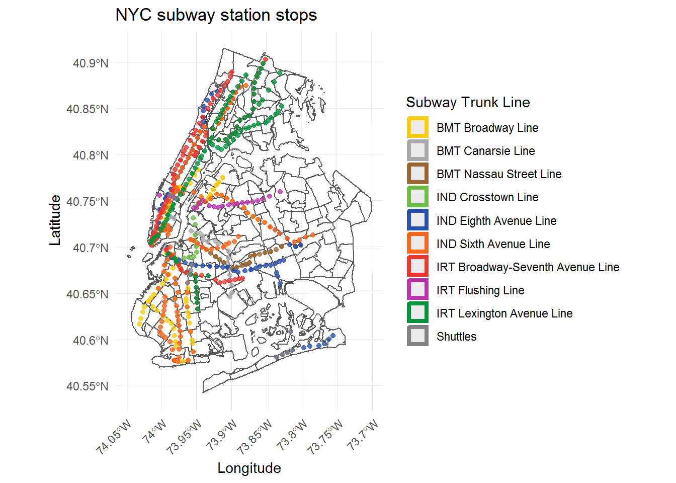

By Route

Let’s first look at how many station stops (ADA-accessible or not) are along each train route.

stat.by.route <- sub.stat.num.updt %>% 
  group_by(route_name) %>% 
  summarize(
    # total number of stations by route:
    total_stat = n(),
    # ada is TRUE/FALSE - use this to get total number of ada stations by route:
    num_ada = sum(ada),
    # percent of total num of station stops that are ada, by route:
    per_ada = round(num_ada * 100 / total_stat, 2)
  ) %>% 
  # convert the 3 shuttles into route_name == "S", to match other datasets
  mutate(rt_mod = ifelse(route_name == "GS" | route_name == "FS" | route_name == "H", "S", route_name)) %>% 
  # join to get subway route groupings, colors
  left_join(sub.line.tidy, by = c("rt_mod" = "route_name")) %>% 
  arrange(primary_trunk_line, route_name)
# create factor for nice route order in plots
stat.by.route$rt_order <- factor(stat.by.route$route_name, levels = stat.by.route$route_name)
# rearrange to match up colors with routes:
subway.by.line <- subway.by.line %>% 
  arrange(primary_trunk_line)

With the summary data frame prepped, it’s time to plot, starting with a bar graph of the total number and the number of ADA-accessible subway station stops by route. The bars will be colored by their traditional NYC subway colors.

# average number of subway stations per route
mean(stat.by.route$total_stat)

[1] 30

stat.by.route %>% 
  ggplot(aes(rt_order, total_stat, fill = primary_trunk_line)) +
  geom_bar(stat = "identity") +
  # dashed line for mean number of total stations
  geom_hline(yintercept = mean(stat.by.route$total_stat), linetype = "dashed") +
  scale_fill_manual(values = subway.by.line$hexadecimal, name = "Trunk Line") +
  ylab("Total number of stations") +
  xlab("Subway route") +
  ggtitle("Total number of subway stations per route")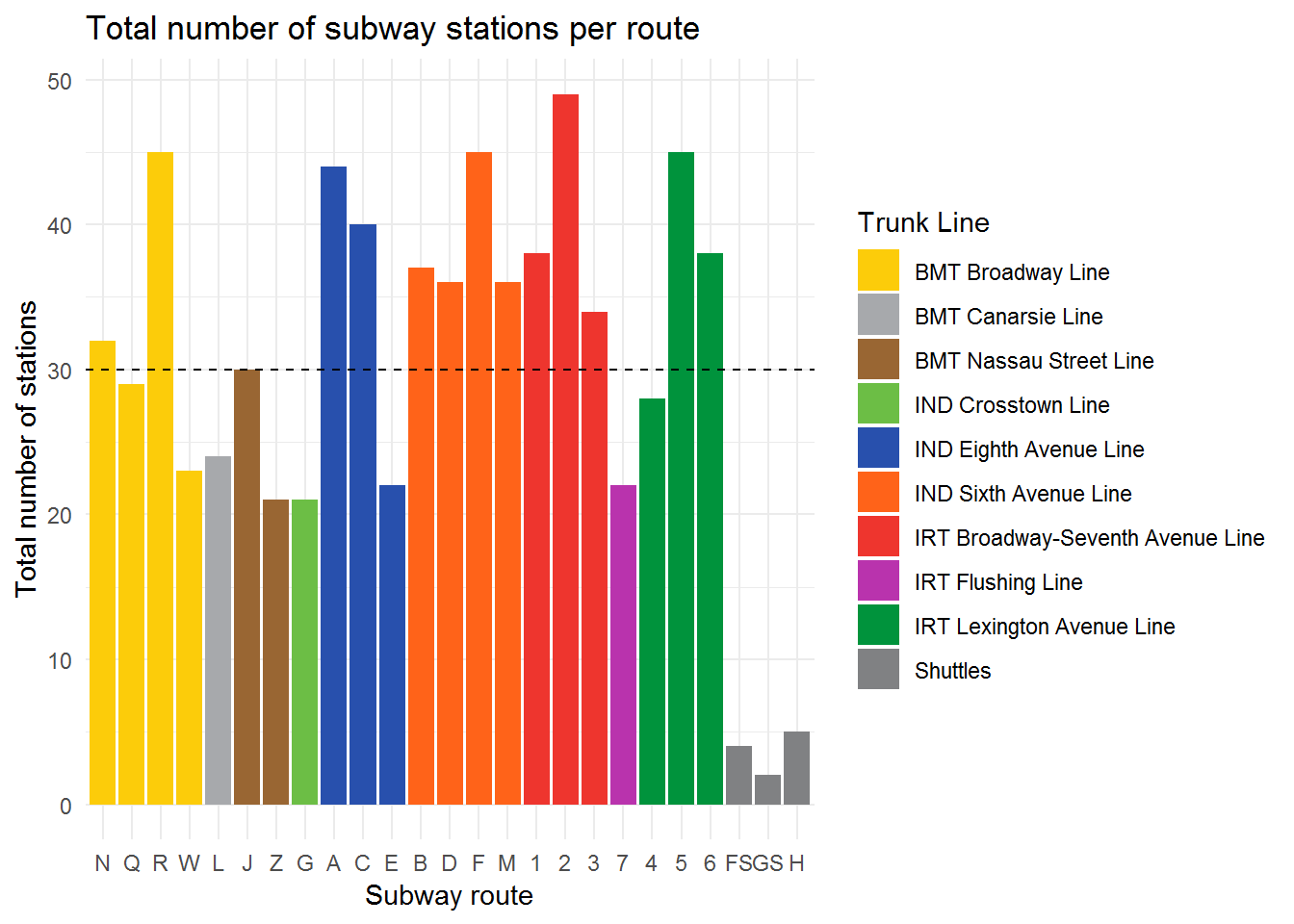

# average number of ada-accessible stations per route:
mean(stat.by.route$num_ada)

[1] 9.12

stat.by.route %>% 
  ggplot(aes(rt_order, num_ada, fill = primary_trunk_line)) +
  geom_bar(stat = "identity") +
  # dashed line for mean number of accessible stations per route
  geom_hline(yintercept = mean(stat.by.route$num_ada), linetype = "dashed") +
  scale_fill_manual(values = subway.by.line$hexadecimal, name = "Trunk Line") +
  ylab("Number of ADA stations") +
  xlab("Subway route") +
  ggtitle("Number of ADA-accessible subway stations per route")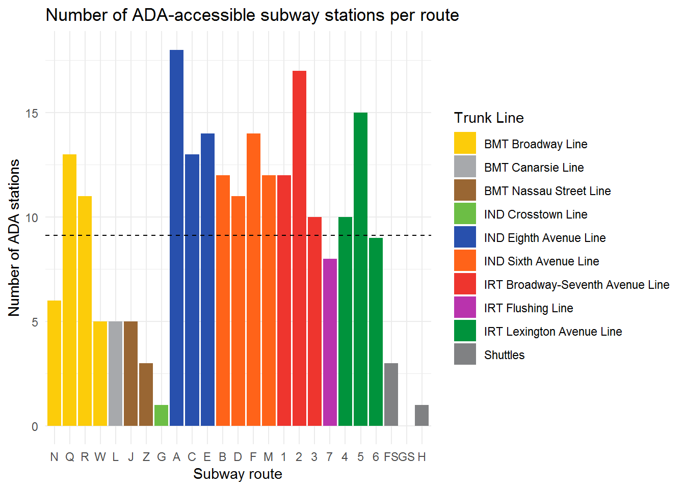

There is an average of 30 stops (of any kind) and 9 ADA-accessible stations per train route; these values are represented by the dashed lines in the plots above.

The number of ADA-accessible stations per route is far less than the total number of stations, which is not unexpected. Let’s take a look at the percent of subway stations that are ADA-accessible per route.

# average percent accessible statious out of total
round(mean(stat.by.route$per_ada), 2)

[1] 30.02

stat.by.route %>% 
  ggplot(aes(rt_order, per_ada, fill = primary_trunk_line)) +
  geom_bar(stat = "identity") +
  geom_hline(yintercept = mean(stat.by.route$per_ada), linetype = "dashed") +
  scale_fill_manual(values = subway.by.line$hexadecimal, name = "Trunk Line") +
  ylab("Percent of stations that are ADA") +
  xlab("Subway route") +
  ggtitle("Percent of ADA-accessible subway stations per route")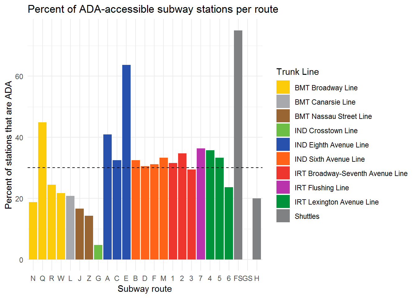

On average, 30% of stations along a subway line are accessible. The Eight Ave, Sixth Ave, Broadway-Seventh Ave, Flushing, and Lexington Ave lines hover close to the mean.

Out of the 25 subway routes, which are worse or better than expected?

# lower accessibility
stat.by.route %>% 
  filter(per_ada < 20) %>% 
  select(route_name:per_ada) %>% 
  arrange(desc(per_ada))

# A tibble: 5 x 4
  route_name total_stat num_ada per_ada
  <chr>           <int>   <int>   <dbl>
1 N                  32       6   18.8 
2 J                  30       5   16.7 
3 Z                  21       3   14.3 
4 G                  21       1    4.76
5 GS                  2       0    0   

# higher accessibility
stat.by.route %>% 
  filter(per_ada > 40) %>% 
  select(route_name:per_ada) %>% 
  arrange(desc(per_ada))

# A tibble: 4 x 4
  route_name total_stat num_ada per_ada
  <chr>           <int>   <int>   <dbl>
1 FS                  4       3    75  
2 E                  22      14    63.6
3 Q                  29      13    44.8
4 A                  44      18    40.9

10 out of the 25 routes have fewer than 25% ADA-accessible station stops, with the N, J, Z, and G suffering from particularly poor accessibility. Only 2 trains, one of which is a shuttle train with 4 stops in total, make it above 50% mark.

I imagine that there should be a superficial relationship between the number of total and accessible stations.

stat.by.route %>% 
  ggplot(aes(total_stat, num_ada, color = primary_trunk_line)) +
  geom_abline(slope = 1, intercept = 0, linetype = "dashed") +
  geom_point(size = 3) +
  scale_color_manual(values = subway.by.line$hexadecimal, name = "Trunk Line") +
  xlim(-5, 55) +
  ylim(-2, 20) +
  xlab("Total number of stations") +
  ylab("Number of ADA stations") +
  ggtitle("Number of ADA-accessible stations vs total number of stations\nPer route")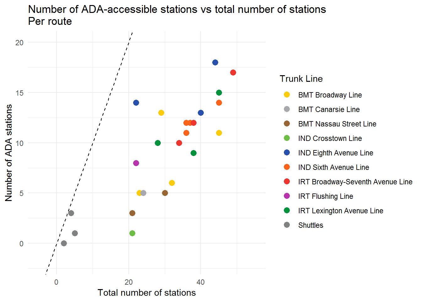

Indeed, the number of ADA-accessible stations does increase with the number of total station stops per route. However, that increase is far less than unity, which is represented by the dashed line in the plot above.

Perhaps for train routes that make more stops, it would be more expensive to have many ADA-accessible stations. What is the relationship between the total number of subway station stops per route with the proportion of stations that are ADA-accessible?

stat.by.route %>% 
  ggplot(aes(total_stat, per_ada, color = primary_trunk_line, label = route_name)) +
  geom_point(size = 3) +
  scale_color_manual(values = subway.by.line$hexadecimal, name = "Trunk Line") +
  geom_text(hjust = 0, vjust = 0, check_overlap = TRUE, nudge_y = 1.5) +
  xlab("Total number of stations") +
  ylab("Percent of stations that are ADA") +
  ggtitle("Percent of ADA-accessible stations vs total number of stations\nPer route")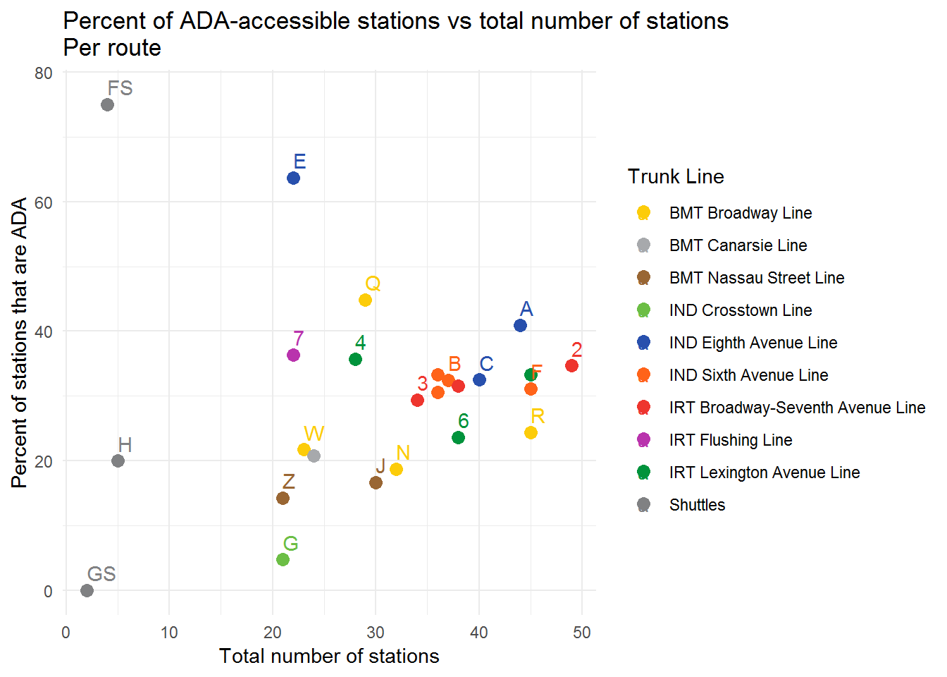

The result is something of a funnel shape with a lot of variation in the lines with fewer stops, and there’s not a clear relationship.

Another visualization method that could be used to compare the total number of stations to the number that are ADA-accessible is a barbell plot. First, the data frame is reordered by the total number of stations per route, to make lines with a similar number of stops easier to compare by eye. Then the total number of stations will be plotted in orange, the number of ADA-accessible stations in blue, and a line segment drawn to connect the two points. The longer the line segment, the greater the difference between the two counts.

stat.by.route <- stat.by.route %>% 
  arrange(total_stat, num_ada) %>% 
  mutate(total_stat_order = factor(route_name, levels = route_name))
stat.by.route %>% 
  ggplot(aes(total_stat_order, total_stat)) +
  geom_segment(aes(x = total_stat_order, xend = total_stat_order, y = num_ada, yend = total_stat), size = 1, alpha= 0.5, color = "gray60") +
  # total number of station stops on route in orange
  geom_point(size = 3, color = "#E69F00") +
  # number of ada-accessible station stops on route in blue
  geom_point(aes(total_stat_order, num_ada), size = 3, color = "#56B4E9") +
  xlab("Route name") +
  ylab("Number of stations") +
  ggtitle("Total number of stations (orange) vs number of ADA-accessible stations (blue)") +
  coord_flip()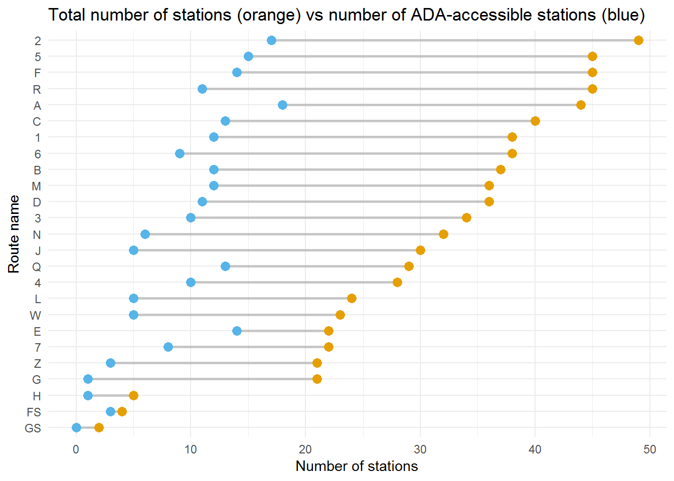

With a barbell plot, it’s possible to make some new observations, such as that the E, 7, Z, and G trains all have about the same number of total stations, but a very different number of ADA-accessible stations.

By Borough

Moving on to the spatial side of things, let’s first explore and compare subway accessibility across the 4 boroughs: Bronx, Brooklyn, Manhattan, and Queens. This is where the sf package starts to become especially useful. Earlier, I had created the object sub.sf.nyc.crs which contains the subway station data and looks like this:

head(sub.sf.nyc.crs)

Simple feature collection with 6 features and 3 fields
geometry type:  POINT
dimension:      XY
bbox:           xmin: 990015.9 ymin: 151802.3 xmax: 1036011 ymax: 213531.4
epsg (SRID):    NA
proj4string:    +proj=lcc +lat_1=40.66666666666666 +lat_2=41.03333333333333 +lat_0=40.16666666666666 +lon_0=-74 +x_0=300000 +y_0=0 +datum=NAD83 +units=us-ft +no_defs
# A tibble: 6 x 4
  stat_name                       ada   route_name                 geometry
  <chr>                           <lgl> <chr>      <POINT [US_survey_foot]>
1 irt_42nd st shuttle_grand cent~ FALSE GS              (990015.9 213531.4)
2 bmt_franklin_botanic gardens    FALSE FS              (995555.6 183503.1)
3 bmt_franklin_park place         TRUE  FS              (996004.5 185116.9)
4 ind_rockaway_beach 105th st     FALSE H                (1032148 151802.3)
5 ind_rockaway_beach 90th st      FALSE H                (1036011 153568.1)
6 ind_rockaway_beach 98th st      FALSE H                (1034091 152570.6)

What is missing now is a borough assignment for each station. While one option would be to find another dataset that matches subway stations to a borough or to try and create complex rules to assign stations by latitude and longitude, instead I can take advantage of the spatial join st_join() function from the sf package. Because subway dataset and the NYC maps now have the same CRS, a spatial join can be used to merge the data based on geometry.

sub.boro <- st_join(sub.sf.nyc.crs, nyc.census.4boro)
head(sub.boro)

Simple feature collection with 6 features and 14 fields
geometry type:  POINT
dimension:      XY
bbox:           xmin: 990015.9 ymin: 151802.3 xmax: 1036011 ymax: 213531.4
epsg (SRID):    NA
proj4string:    +proj=lcc +lat_1=40.66666666666666 +lat_2=41.03333333333333 +lat_0=40.16666666666666 +lon_0=-74 +x_0=300000 +y_0=0 +datum=NAD83 +units=us-ft +no_defs
# A tibble: 6 x 15
  stat_name ada   route_name ctlabel borocode boroname ct2010 boroct2010
  <chr>     <lgl> <chr>      <fct>   <fct>    <fct>    <fct>  <fct>     
1 irt_42nd~ FALSE GS         94      1        Manhatt~ 009400 1009400   
2 bmt_fran~ FALSE FS         213     3        Brooklyn 021300 3021300   
3 bmt_fran~ TRUE  FS         305     3        Brooklyn 030500 3030500   
4 ind_rock~ FALSE H          938     4        Queens   093800 4093800   
5 ind_rock~ FALSE H          942.02  4        Queens   094202 4094202   
6 ind_rock~ FALSE H          942.01  4        Queens   094201 4094201   
# ... with 7 more variables: cdeligibil <fct>, ntacode <fct>,
#   ntaname <fct>, puma <fct>, shape_leng <dbl>, shape_area <dbl>,
#   geometry <POINT [US_survey_foot]>

All of the information that was in the NYC census shapefile has been merged with the subway station stops data. For now, since the focus of this section is only on the borough summary data, I’ll drop the geometry information and columns relating to neighborhoods and census tracts.

sub.boro.nogeo <- sub.boro %>% 
  # get rid of geometry, turn back to just a data frame:
  st_set_geometry(NULL) %>% 
  as_tibble() %>% 
  select(stat_name:route_name, boroname:boroct2010, ntaname, shape_area)
# preview of new df:
head(sub.boro.nogeo)

# A tibble: 6 x 8
  stat_name  ada   route_name boroname ct2010 boroct2010 ntaname shape_area
  <chr>      <lgl> <chr>      <fct>    <fct>  <fct>      <fct>        <dbl>
1 irt_42nd ~ FALSE GS         Manhatt~ 009400 1009400    Midtow~   1646379.
2 bmt_frank~ FALSE FS         Brooklyn 021300 3021300    Crown ~   1989395.
3 bmt_frank~ TRUE  FS         Brooklyn 030500 3030500    Crown ~   3474329.
4 ind_rocka~ FALSE H          Queens   093800 4093800    Breezy~   8701238.
5 ind_rocka~ FALSE H          Queens   094202 4094202    Hammel~   7609021.
6 ind_rocka~ FALSE H          Queens   094201 4094201    Breezy~   3813369.

# group by and summrize station-route counts by borough:
boro.stat.count <- sub.boro.nogeo %>%
  group_by(boroname) %>% 
  summarize(
    # total number of station stops
    tot_stat = n(),
    # ada station stop count
    ada_stat = sum(ada),
    not_ada = tot_stat - ada_stat,
    # percet of stations that are ada:
    ada_percent = ada_stat * 100 / tot_stat
    ) %>% 
  # order by station count, from most to least
  arrange(desc(tot_stat)) %>% 
  mutate(tot_plot_ord = factor(boroname, levels = boroname, labels = c("Manhattan", "Brooklyn", "Queens", "Bronx")))

An important reminder is that even though I refer to them as “station stops,” technically what I am counting is distinct subway station stop and subway route associations per borough. In other words, I’m not only counting how many subway stations there are, but what I’m actually summing up is each train that stops at that station. For example, the Times Square subway station adds 9 to the tot_stat variable because 9 routes service it (Port Authority, where 3 more trains stop, is treated as a separate station) and 8 to the ada_stat variable (GS is not ADA-accessible) for Manhattan. Again, as I have mentioned earlier, I am counting the station stops in this way because I would argue that the more trains stop somewhere, the more “accessible” or “reachable” the area is, and this method of counting is my way of including that idea in the analysis.

With that disclaimer out of the way, let’s look at the subway station stop counts by borough.

boro.stat.count %>% 
  ggplot(aes(tot_plot_ord, tot_stat, fill = tot_plot_ord)) + 
  geom_bar(stat= "identity") +
  scale_fill_tableau() +
  xlab("Borough") +
  ylab("Total number of stations") +
  theme(legend.position = "none") +
  ggtitle("Subway station stop count per borough")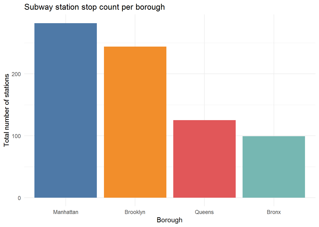

Perhaps unsurprisingly, Manhattan has the highest count of subway stations stops, followed by Brooklyn, then Queens and lastly the Bronx. Even though more people live in Brooklyn and Queens, Manhattan is arguably the tourist and economic hub of the city where many people visit and work. Another reason why the station count is highest in Manhattan is that all trains, except for the G and the FS and H shuttles, cross through or start/end in Manhattan.

What about the number of ADA-accessible subway stations across the boroughs?

# dodge view
boro.stat.count %>% 
  select(-c(tot_stat, ada_percent)) %>% 
  gather("stat_type", "num_stat", ada_stat:not_ada) %>% 
  mutate(stat_type = ifelse(stat_type == "ada_stat", "ADA Station", "Not ADA")) %>% 
  ggplot(aes(tot_plot_ord, num_stat, fill = stat_type)) +
  geom_bar(stat = "identity", position = "dodge") +
  scale_fill_tableau(name = "Station Type") +
  xlab("Borough") +
  ylab("Number of subway stations") +
  ggtitle("Station stop count by borough")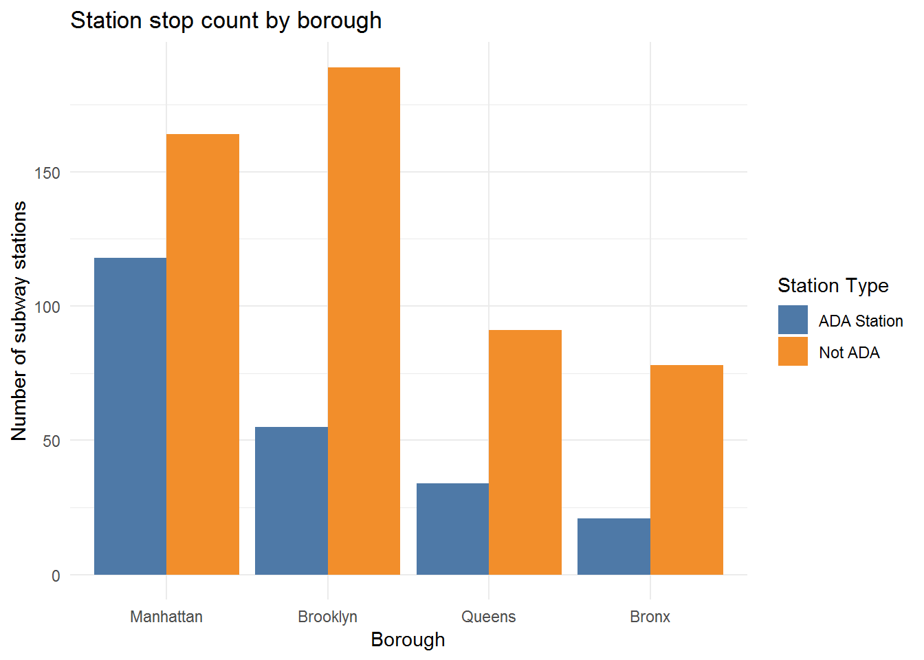

# fill view
boro.stat.count %>% 
  select(-c(tot_stat, ada_percent)) %>% 
  gather("stat_type", "num_stat", ada_stat:not_ada) %>% 
  mutate(stat_type = ifelse(stat_type == "ada_stat", "ADA Station", "Not ADA")) %>% 
  ggplot(aes(tot_plot_ord, num_stat, fill = stat_type)) +
  geom_bar(stat = "identity", position = "fill") +
  scale_fill_tableau(name = "Station Type") +
  xlab("Borough") +
  ylab("Proportion") +
  ggtitle("Station stop count by borough\n(Bar Fill)")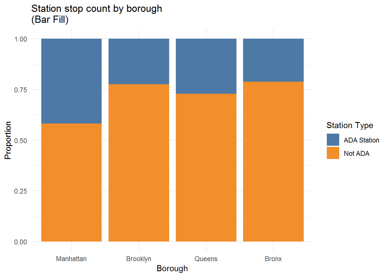

Manhattan has by far, the highest number of accessible subway route stations. The proportion of ADA-accessible stations is higher in Manhattan than in the other 3 boroughs as well.

By Neighborhood

Now to zoom in a bit more in terms of spatial scale, let’s look at subway station stops by neighborhood and finally approach one of the primary aims of this project, which is to recreate the accessibility map featured in the NYC Comptroller report.

The data frame that was created for the borough comparison will be used again, but this time the summary statistics will be calculated on a smaller geographical scale with a neighborhood grouping. The group_by() call will also include the boroughs, which does not add to the groups because the neighborhood names in the ntanames column are unique, but it is an easy way to carry along the borough-neighborhood data for analysis down the line.

neigh.stat.count <- sub.boro.nogeo %>% 
  # grouping by borough allows for that column to be carried along:
  group_by(boroname, ntaname) %>% 
  summarize(
    tot_stat = n(),
    ada_stat = sum(ada),
    not_ada = tot_stat - ada_stat,
    ada_percent = round(ada_stat * 100 / tot_stat, 2)
    ) %>%
  ungroup() %>% 
  # add in neighborhoods with no subway stations
  bind_rows(
    nyc.neigh.4boro %>% 
    st_set_geometry(NULL) %>% 
    as_tibble() %>% 
    filter(!(ntaname %in% sub.boro.nogeo$ntaname)) %>% 
    select(boroname, ntaname) %>% 
    mutate(
      tot_stat = 0,
      ada_stat = 0,
      not_ada = 0, 
      ada_percent = NA
    )
  ) %>% 
  # plot order column, same order as for the borough analysis (total count)
  mutate(boro_order = factor(boroname, levels = boro.stat.count$boroname, labels = c("Manhattan", "Brooklyn", "Queens", "Bronx"))) 

# calculate some summary stats:
neigh.stat.count %>% 
  group_by(boro_order) %>% 
  summarize(
    # mean subway station stops per neighbohood for each borough
    mean_sub_stat = mean(tot_stat),
    # median subway station stops per neighbohood for each borough
    med_sub_stat = median(tot_stat),
    # mean ADA-accessible subway station stops per neighbohood for each borough
    mean_ada_stat = mean(ada_stat),
    # mean ADA-accessible subway station stops per neighbohood for each borough
    med_ada_stat = median(ada_stat)
    )

# A tibble: 4 x 5
  boro_order mean_sub_stat med_sub_stat mean_ada_stat med_ada_stat
  <fct>              <dbl>        <dbl>         <dbl>        <dbl>
1 Manhattan           9.72            6         4.07             2
2 Brooklyn            4.78            4         1.08             0
3 Queens              2.16            0         0.586            0
4 Bronx               2.61            2         0.553            0

Looking at the borough averages for the number of total and ADA-accessible subway station stops per neighborhood reinforces the conclusion from the previous section that Manhattan has, on average, the highest count of both. The difference between the means and medians suggests that the distribution of this data might be at least slightly skewed, but let’s take a closer look at the distributions.

Violin plots are helpful tools for precisely that purpose. If you’re not familiar with this plot style, think of it as a density plot reflected across the x-axis and flipped sideways. The following violin plots were inspired by the STHDA violin plot tutorial, which has many helpful guides on ggplot2 (as well as other topics). The data_summary() function is used to plot the mean and the standard deviation over the violin plots to provide more information about the distribution of the data.

data_summary <- function(x) {
   m <- mean(x)
   ymin <- m - sd(x)
   ymax <- m + sd(x)
   return(c(y = m, ymin = ymin, ymax = ymax))
}
neigh.stat.count %>% 
  ggplot(aes(boro_order, tot_stat, color = boro_order, fill = boro_order)) +
  geom_violin() +
  stat_summary(fun.data = data_summary, color = "black", alpha = 0.8) +
  scale_color_tableau() +
  scale_fill_tableau() +
  xlab("Borough") +
  ylab("Count per neighborhood") +
  theme(legend.position = "none") +
  ggtitle("Number of subway station stops within a neighborhood\nAll stations")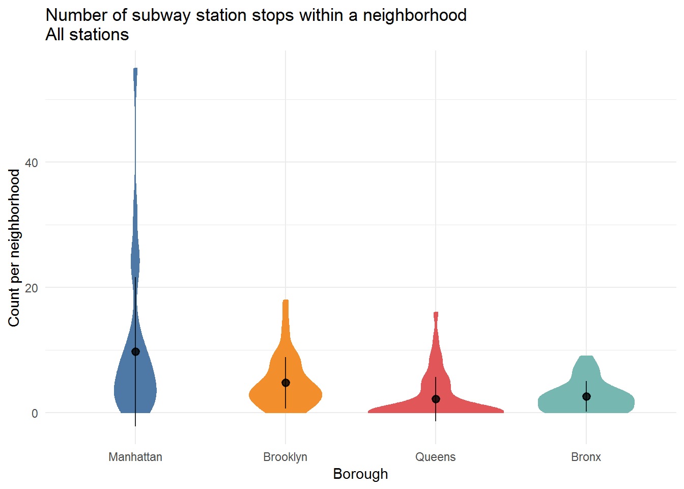

neigh.stat.count %>% 
  ggplot(aes(boro_order, ada_stat, color = boro_order, fill = boro_order)) +
  geom_violin() +
  stat_summary(fun.data = data_summary, color = "black", alpha = 0.8) +
  scale_color_tableau() +
  scale_fill_tableau() +
  xlab("Borough") +
  ylab("Count per neighborhood") +
  theme(legend.position = "none") +
  ggtitle("Number of subway station stops within a neighborhood\nADA-accessible stations only")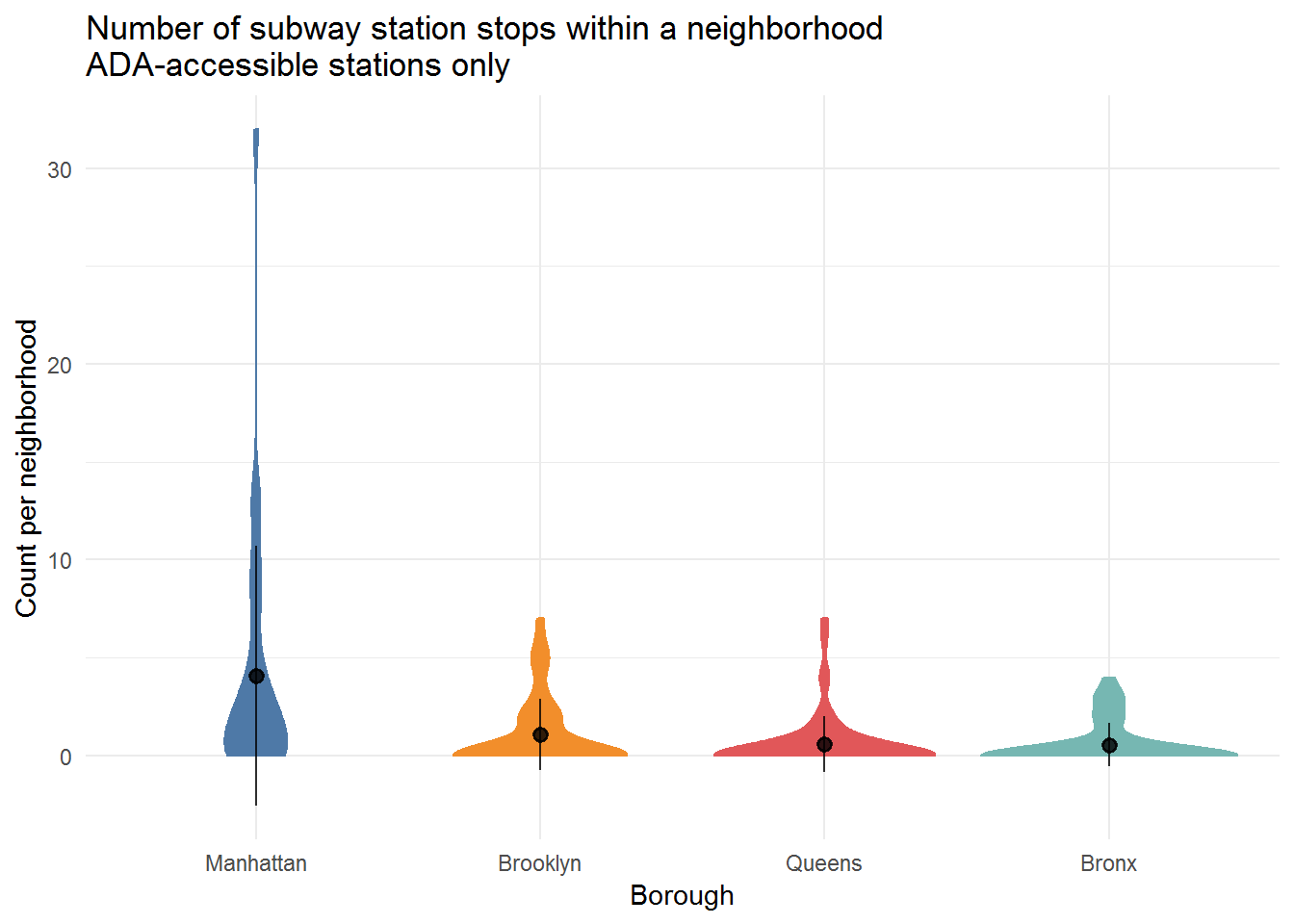

The distributions for both types of stations are right-skewed, with the Manhattan neighborhood counts having the longest tail, which means that there is a small number of neighborhoods with a high station stop count. A heavy distribution towards zero, such as the Bronx data in either plot, indicates that these boroughs have very few subway station stops per neighborhood.

The distributions of the percent of ADA-accessible station stops per neighborhood, on the other hand, are more on the uniform side, although still right skewed for Brooklyn and the Bronx (values are NA for neighborhoods with no subway stations and are not included).

neigh.stat.count %>% 
  ggplot(aes(boro_order, ada_percent, color = boro_order, fill = boro_order)) +
  geom_violin() +
  stat_summary(fun.data = data_summary, color = "black", alpha = 0.8) +
  scale_color_tableau() +
  scale_fill_tableau() +
  xlab("Borough") +
  ylab("Percent per neighborhood") +
  theme(legend.position = "none") +
  ggtitle("Percent of ADA-accessible subway station stops within a neighborhood")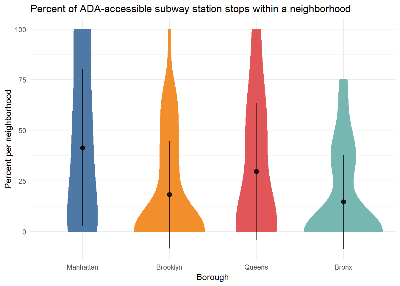

Both the distribution of the station stop counts and the neighborhood land areas are right skewed:

neigh.stat.count %>% 
  select(-c(not_ada:boro_order)) %>% 
  rename(`Total Stations` = tot_stat, `ADA-accessible Stations` = ada_stat) %>% 
  gather(key = "count_type", value = "n", `Total Stations`:`ADA-accessible Stations`) %>% 
  ggplot(aes(n, fill = count_type)) +
  geom_histogram(bins = 30) +
  facet_wrap(~ count_type) +
  scale_fill_tableau(name = "Station Type") +
  xlab("Number of station stops per neighborhood") +
  ylab("Count")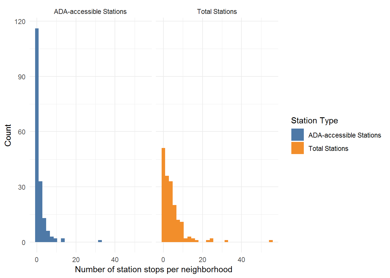

nyc.neigh.4boro %>% 
  filter(!(str_detect(ntaname, "park") | str_detect(ntaname, "Airport"))) %>% 
  ggplot(aes(shape_area)) +
  geom_histogram(bins = 30) +
  xlab("Neighborhood area (sq ft)") +
  ylab("Count") +
  ggtitle("Neighborhood land area")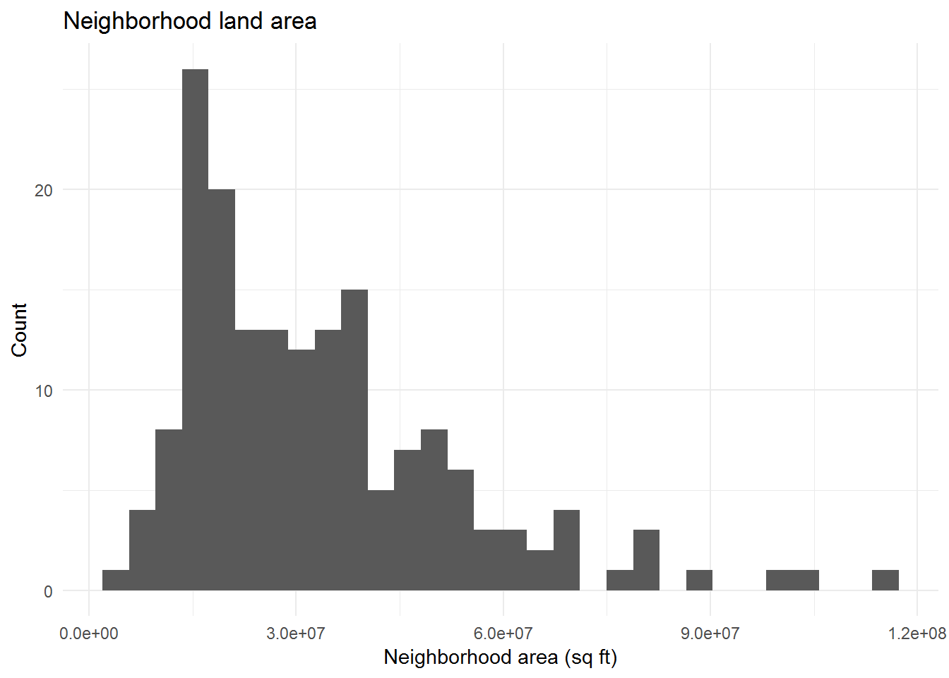

Perhaps the distributions of subway stop counts would be more normal if the counts were divided by neighborhood area?

neigh.stat.count %>% 
  inner_join(nyc.neigh.4boro, by = "ntaname") %>% 
  select(boro_order, ntaname:ada_percent, shape_area) %>%
  mutate(
    # convert neighborhood area from sq ft to sq miles (friendlier unit)
    area_mi = shape_area / 5280**2,
    # divide stop counts by neighborhood area in sq miles
    `Total Stations` = tot_stat / area_mi,
    `ADA-accessible Stations` = ada_stat / area_mi
    ) %>% 
  select(boro_order, `Total Stations`:`ADA-accessible Stations`) %>% 
  gather("stat_type", "per_sqmi", `Total Stations`:`ADA-accessible Stations`) %>% 
  ggplot(aes(boro_order, per_sqmi, color = boro_order, fill = boro_order)) +
  geom_violin() +
  scale_fill_tableau() +
  scale_color_tableau() +
  facet_wrap(~ stat_type, ncol = 2) +
  stat_summary(fun.data = data_summary, color = "black", alpha = 0.8) +
  theme(legend.position = "none") +
  xlab("Borough") +
  ylab("Number of station stops per sq mile") +
  ggtitle("Station stop count per square mile per neighborhood")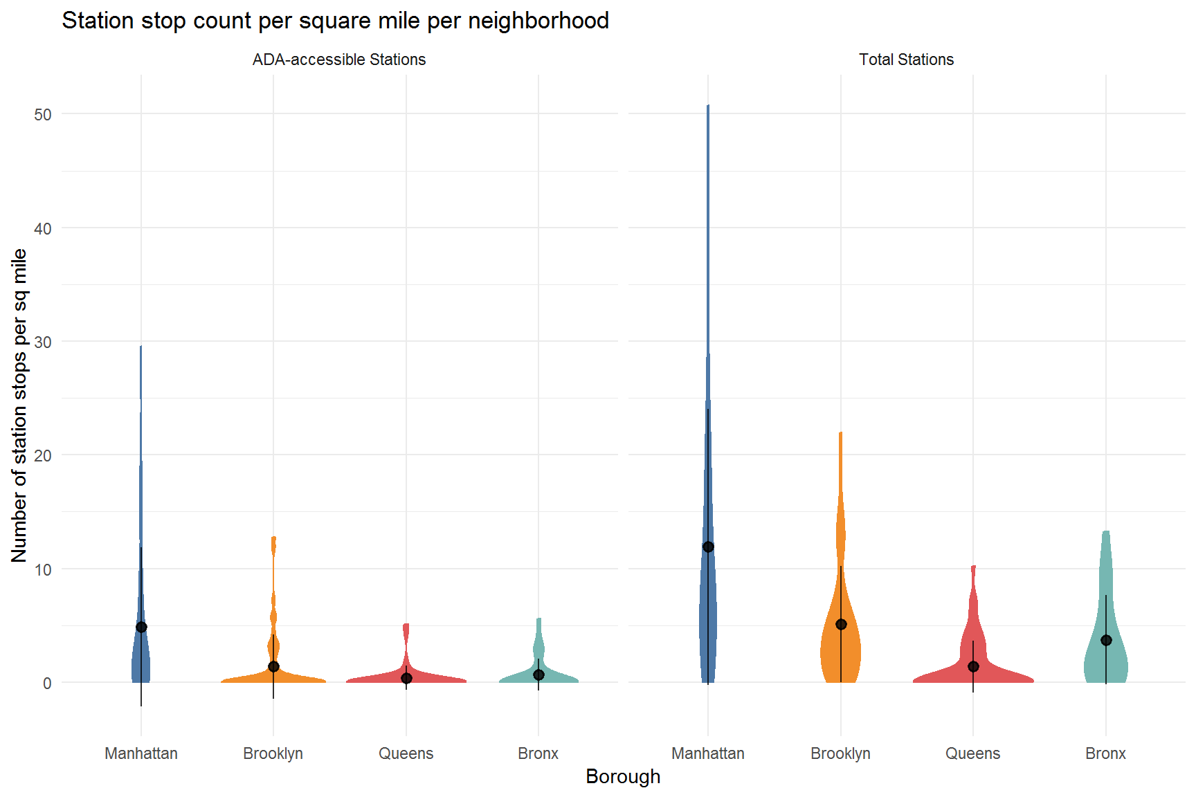

Looks like there’s still a strong right skew in the resulting data.

Now it’s time to switch tracks and recreate the NYC map such that each neighborhood is filled based on whether or not there is an accessible station. First, the (non-spatial) summary data frame of station stops per neighborhood will be joined onto the NYC neighborhood shapefile. Then, the case_when() function will be used to create a new group column. I discovered case_when() recently as an alternative to nested ifelse() function calls and find them to be easier to read in many situations.

nyc.neigh.4boro.count <- nyc.neigh.4boro %>% 
  full_join(
    neigh.stat.count %>% 
      select(-boroname) %>% 
      # filter out neigh with no stations for mapping purposes
      filter(ntaname %in% sub.boro.nogeo$ntaname),
    by = "ntaname"
  )
neigh.map.count.prep <- nyc.neigh.4boro.count %>% 
  # create column to fill neighborhoods on map by
  mutate(
    neigh_group = case_when(
      # Park group:
      str_detect(ntaname, "park") ~ "Park", 
      # Airport:
      str_detect(ntaname, "Airport") ~ "Airport", 
      # Neither park nor airport, and no subway stations at all
      !(str_detect(ntaname, "park") | str_detect(ntaname, "Airport")) & is.na(tot_stat) ~ "No stations", 
      # Neither park nor airport, has subway stations, but no ADA stations:
      !(str_detect(ntaname, "park") | str_detect(ntaname, "Airport")) & tot_stat > 0 & ada_stat < 1 ~ "No accessible stations", 
      # Neither park nor airport, has at least 1 ADA station:
      !(str_detect(ntaname, "park") | str_detect(ntaname, "Airport")) & tot_stat > 0 & ada_stat > 0 ~ "At least one accessible station", 
      # else statement, sign of something wrong in the logic: 
      TRUE ~ "Don't know"
      )
  )
# resulting breakdown for neighborhoods:
table(neigh.map.count.prep$neigh_group)

                        Airport At least one accessible station 
                              1                              58 
         No accessible stations                     No stations 
                             63                              50 
                           Park 
                              4 

# Map:
neigh.map.count.prep %>% 
  ggplot() +
  geom_sf(aes(fill = neigh_group), color = "#BFBFBF") +
  scale_fill_manual(values = c("grey30", "#0072B2", "#E69F00", "#999999", "#bae4b3"), name = "Neighborhood Type") + 
  # overlay subway:
  geom_sf(data = sub.sf.nyc.crs, color = "grey80", fill = "black", size = 2, pch = 21) +
  theme(axis.text.x = element_blank(), axis.text.y = element_blank()) +
  ggtitle("Neighborhoods with no accessible subway station")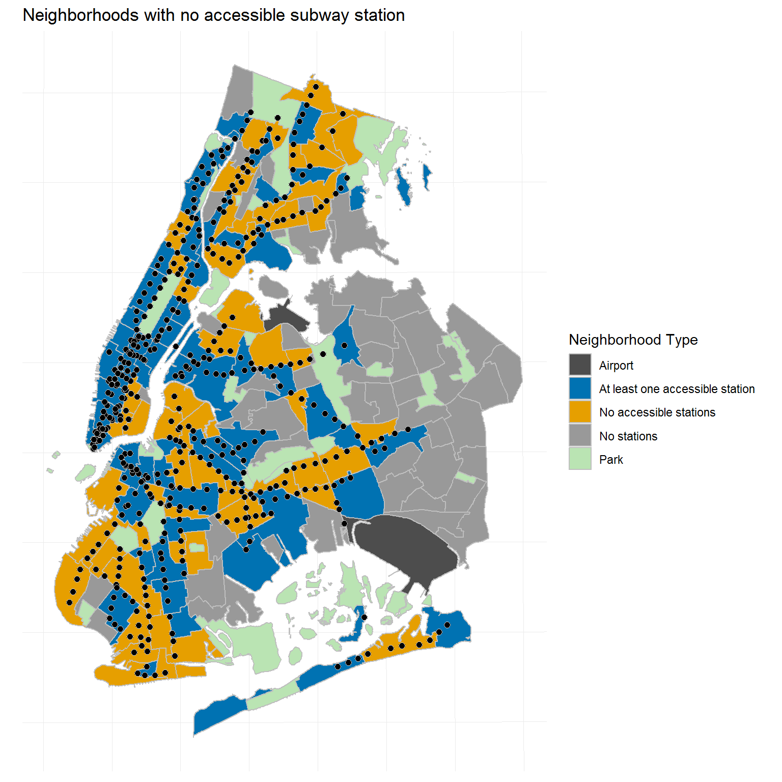

And there we are! Not a perfect replica, but pretty darn close. I also chose to explicitly block out the two airports as well, which was not the case in the Comptroller report map.

The advantage of this project format is that I can also include interactive figures, so here’s one where you can switch background maps and explore the neighborhoods to see their names, borough, and station stop counts.

neigh.map.count.prep %>%
  rename(`Neighborhood Type` = neigh_group) %>% 
  select(boroname, ntaname, ntacode, `Neighborhood Type`, tot_stat:ada_percent) %>% 
  mapview(zcol = "Neighborhood Type", col.regions = c("grey30", "#0072B2", "#E69F00", "#999999", "#bae4b3"))

One discrepancy between the original map and my recreation is that the East Harlem South neighborhood (located in Manhattan, east of Central Park) was marked as having an ADA-accessible station in the report map, whereas on mine it does not. This is likely due to a slight difference in the coordinates that were used for the Q train 96th St stop, which is on the border of East Harlem South and the Yorkville neighborhood to the south of East Harlem.

Let’s now look at a map of the station counts. In the previous plot of NYC, I blocked out the parks and airports using a separate column assignment, but the ggplot2 principle of layering objects can also be used with a subset of the shapefile to avoid mixing characters and numbers in the same column when working with numeric data.

nyc.parks.air.sf <- nyc.census.4boro %>% 
  filter(str_detect(ntaname, "park") | str_detect(ntaname, "Airport"))
neigh.map.count.prep %>%
  ggplot() +
  geom_sf(aes(fill = tot_stat), color = "black") +
  scale_fill_viridis_c(option = "D", name = "Count") +
  # overlay parks and airports
  geom_sf(data = nyc.parks.air.sf, fill =  "grey30", color = "black") +
  theme(axis.text.x = element_blank(), axis.text.y = element_blank()) +
  ggtitle("Number of subway station stops within neighborhood\nAll stations")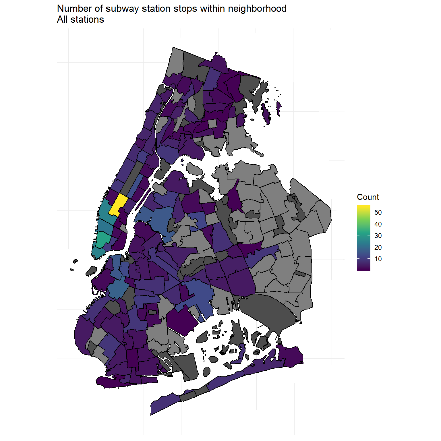

Ah, but that map is not exactly informative because, as seen earlier, the subway stop count distribution is highly right-skewed. A solution is to convert the continuous numeric count value into a discrete factor using the cut() and quantile() functions to break the numbers into 4 bins that each contain about 25% of the data.

neigh.map.count.prep %>% 
  mutate(tot_fact = cut(tot_stat, quantile(tot_stat, na.rm = TRUE), include.lowest = TRUE)) %>% 
  ggplot() +
  geom_sf(aes(fill = tot_fact), color = "black") +
  scale_fill_viridis_d(option = "D", name = "Count Quantiles", na.value = "gray50") +
  geom_sf(data = nyc.parks.air.sf, fill =  "grey30", color = "black") +
  theme(axis.text.x = element_blank(), axis.text.y = element_blank()) +
  ggtitle("Number of subway station stops within neighborhood\nAll stations")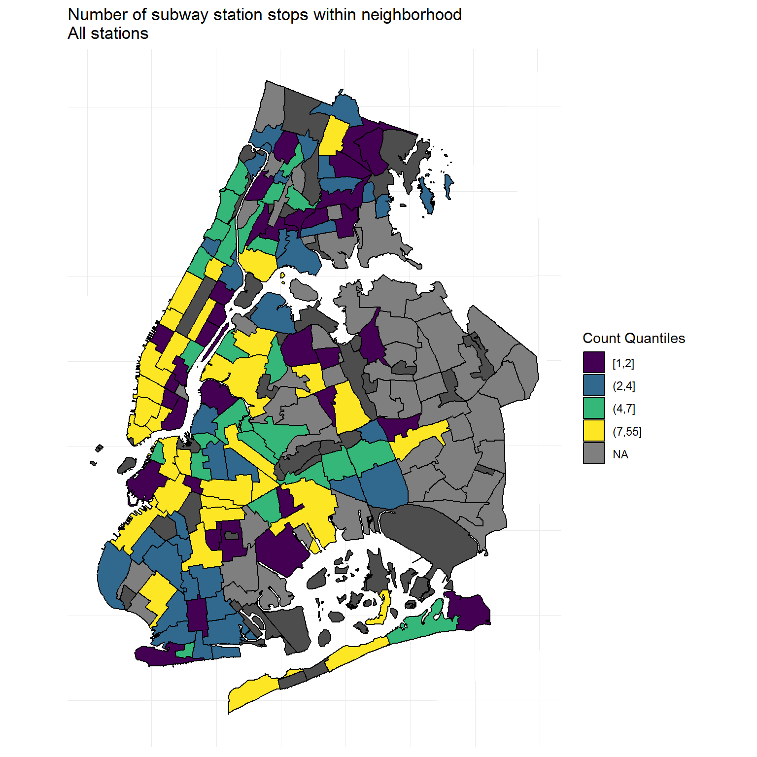

neigh.map.count.prep %>% 
  mutate(
    ada_stat = ifelse(ada_stat == 0, NA, ada_stat),
    ada_fact = cut(ada_stat, quantile(ada_stat, na.rm = TRUE), include.lowest = TRUE)
    ) %>% 
  ggplot() +
  geom_sf(aes(fill = ada_fact), color = "black") +
  scale_fill_viridis_d(option = "D", name = "Count Quantiles", na.value = "gray50") +
  geom_sf(data = nyc.parks.air.sf, fill =  "grey30", color = "black") +
  theme(axis.text.x = element_blank(), axis.text.y = element_blank()) +
  ggtitle("Number of subway station stops within neighborhood\nADA-accessible stations only")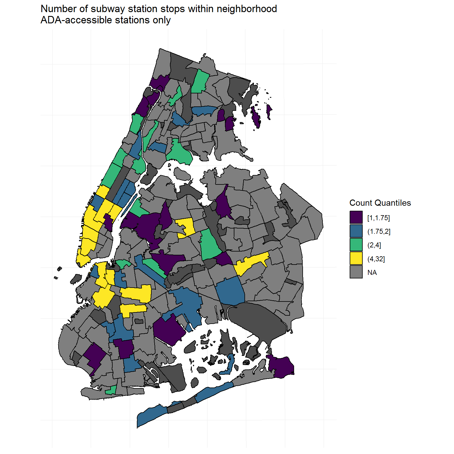

The raw counts may not be the most helpful way of looking at the data, but the percentage of stations that are ADA-accessible could be more informative in trying to understand which areas are underserviced specifically by accessible subway stations. It would be unrealistic to expect new stations to be built, but existing stations could be converted to meet ADA requirements.

To specifically highlight areas that are 0% accessible, they will be filled with a separate color, just like in the report, and the percent ADA-accessible values will be turned into a factor by binning the values with breaks every 20%.

nyc.neigh.notada <- neigh.map.count.prep %>% 
  filter(ada_stat == 0)
neigh.map.count.prep <- neigh.map.count.prep %>% 
  mutate(ada_percent = ifelse(ada_percent == 0, NA, ada_percent))
neigh.map.count.prep$ada_per_breaks <- as.character(cut(neigh.map.count.prep$ada_percent, breaks = seq(0, 100, 20)))
neigh.map.count.prep <- neigh.map.count.prep %>% 
  # insert the neighborhoods with subway stations (not ADA) into the fill code:
  mutate(
    ada_per_breaks = case_when(
      ntacode %in% nyc.parks.air.sf$ntacode ~ "Park / Airport",
      ntacode %in% nyc.neigh.notada$ntacode ~ "No accessible stations",
      TRUE ~ ada_per_breaks
      )
    ) 
neigh.map.count.prep %>% 
  ggplot() +
  geom_sf(aes(fill = ada_per_breaks), color = "black") +
  scale_fill_manual(values = c("#c7e9b4", "#7fcdbb", "#41b6c4", "#2c7fb8", "#253494", "#b8652c", "grey30"), na.value = "gray50", name = "Percent ADA Breaks") + 
  theme(axis.text.x = element_blank(), axis.text.y = element_blank()) +
  ggtitle("Percent of ADA-accessible subway station stops\nPer Neighborhood")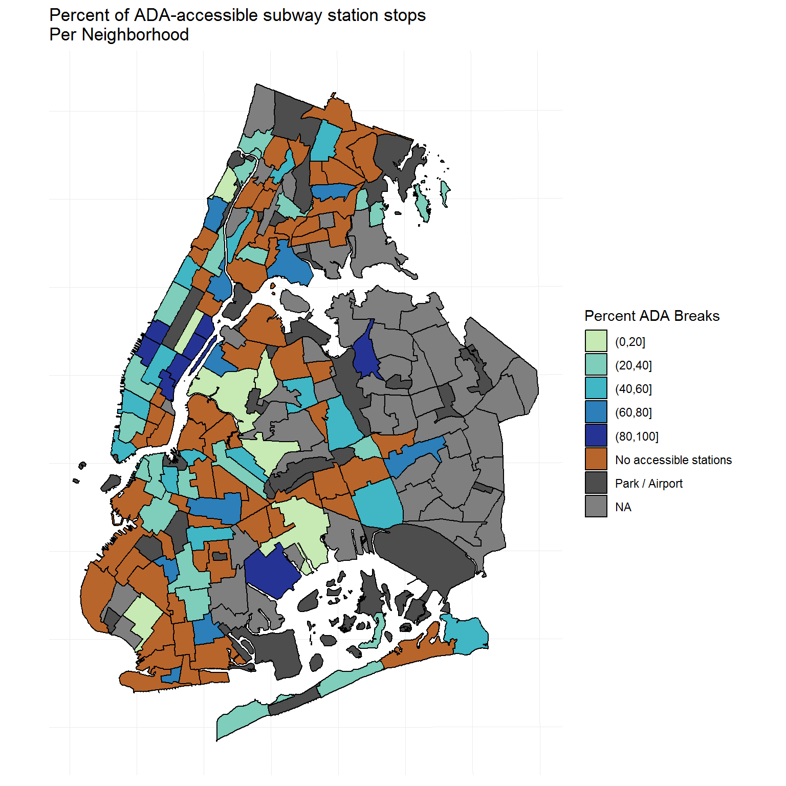

And, of course, here is the interactive version (because why not).

neigh.map.count.prep %>% 
  # need to replace for the color fill to work correctly with mapview:
  mutate(ada_per_breaks = replace_na(ada_per_breaks, "No stations")) %>% 
  select(boroname, ntaname, ntacode, ada_per_breaks, tot_stat:ada_percent) %>% 
  rename(`Percent ADA-Accessible` = ada_per_breaks) %>% 
  mapview(
    zcol = "Percent ADA-Accessible",
    col.regions = c("#c7e9b4", "#7fcdbb", "#41b6c4", "#2c7fb8", "#253494", "#b8652c", "gray50", "grey20")
    )

Census tract buffer analysis

Let’s pivot to the census tracts and zoom in even more in geospatial terms. The tracts themselves are too small in area to learn something useful by simply counting the number of stations within the area of each tract. Instead, I will use buffer analysis to determine how many stations are within a certain range from each census tract center.

First, the center of each tract can be found using the st_centroid() function from the sf package:

tract.cent <- st_centroid(nyc.census.4boro)
# result mapped: 
nyc.census.4boro %>% 
  ggplot() +
  geom_sf(color = "#BFBFBF") +
  geom_sf(data = tract.cent, size = 0.75, color = "#4E79A7") +
  ggtitle("NYC census tract centroids") + 
  theme(axis.text.x = element_blank(), axis.text.y = element_blank())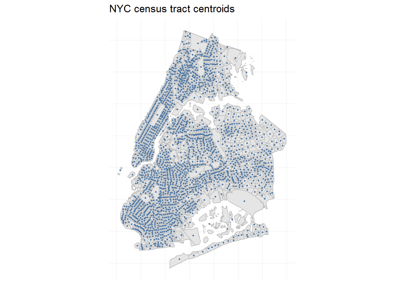

Then, those centroid points can be used as the center to draw a circle with a chosen radius, specified in feet with the dist argument in the st_buffer() function call below. I chose to draw buffers with a half-mile radius, or 2,640 ft, which may even be too generous of a radius for someone who has certain accessibility needs, but it’s a start.

The resulting geometry is too chaotic to map all at once, but I can select two census tracts to demonstrate as an example.

# create a half-mile buffer around every centroid:
tract.cent.halfmi.buff <- st_buffer(tract.cent, dist = 2640)
#example
nyc.census.4boro %>% 
  ggplot() +
  geom_sf(color = "#BFBFBF") +
  geom_sf(
    data = tract.cent.halfmi.buff %>%
      # pick 2 census tracts as examples:
      filter(boroct2010 == 1009800 | boroct2010 == 1018400),
    alpha = 0.8, color = "#F28E2B", fill = "#F28E2B"
    ) +
  # overlay subway station locations:
  geom_sf(data = sub.sf.nyc.crs, color = "black", size = 0.75) +
  ggtitle("Centroid buffer example\n0.5 buffer mile radius") +
  theme(axis.text.x = element_blank(), axis.text.y = element_blank())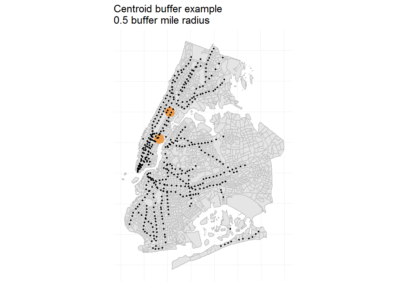

Above are two examples of buffers drawn as orange circles, with the subway stations overlaid in black. These new spatial objects inherited the geometry from the NYC tract maps, and have the same properties as other sf objects. From here, it’s only a matter of using a spatial join to determine how many subway station stops fall into each buffer.

Below is an example of the join for the northern buffer, the one that’s at the top of Central Park. This buffer captures 5 separate subway stations, 2 for the red line and 3 for the green line, and all of the trains that stop at those stations.

st_join(sub.sf.nyc.crs, tract.cent.halfmi.buff) %>% 
  st_set_geometry(NULL) %>% 
  filter(boroct2010 == 1018400) %>% 
  select(stat_name:route_name, boroct2010) %>% 
  arrange(stat_name, route_name)

# A tibble: 9 x 4
  stat_name                             ada   route_name boroct2010
  <chr>                                 <lgl> <chr>      <fct>     
1 irt_lenox_110th st-central park north FALSE 2          1018400   
2 irt_lenox_110th st-central park north FALSE 3          1018400   
3 irt_lenox_116th st                    FALSE 2          1018400   
4 irt_lenox_116th st                    FALSE 3          1018400   
5 irt_lexington_110th st                FALSE 6          1018400   
6 irt_lexington_116th st                FALSE 6          1018400   
7 irt_lexington_125th st                TRUE  4          1018400   
8 irt_lexington_125th st                TRUE  5          1018400   
9 irt_lexington_125th st                TRUE  6          1018400   

Multiple trains stop at most of these stations and so I would then count that the census tract associated with this buffer is in range of 9 subway station route stops, 3 of which are ADA-accessible.

The actual join will be broken up by borough, because all boroughs, except for Brooklyn and Queens, are separated by water.

sub.sf.nyc.crs.boro <- sub.sf.nyc.crs %>% 
  inner_join(
    sub.boro.nogeo %>% 
      select(stat_name, boroname) %>% 
      distinct(),
    by = "stat_name"
  )
sub.join.borolim <- sub.sf.nyc.crs.boro %>% 
  # manhattan
  filter(boroname == "Manhattan") %>% 
  st_join(
    tract.cent.halfmi.buff %>% 
      filter(boroname == "Manhattan")
    ) %>% 
  st_set_geometry(NULL) %>% 
  bind_rows(
    # bronx
    sub.sf.nyc.crs.boro %>% 
      filter(boroname == "Bronx") %>% 
      st_join(
        tract.cent.halfmi.buff %>% 
          filter(boroname == "Bronx")
        ) %>% 
      st_set_geometry(NULL)
    ) %>% 
  bind_rows(
    # brooklyn and queens together
    sub.sf.nyc.crs.boro %>% 
      filter(boroname == "Brooklyn" | boroname == "Queens") %>% 
      st_join(
        tract.cent.halfmi.buff %>% 
          filter(boroname == "Brooklyn" | boroname == "Queens")
        ) %>% 
      st_set_geometry(NULL)
    )

nyc.4boro.buff.join <- nyc.census.4boro %>% 
  full_join(
    sub.join.borolim %>% 
      group_by(boroct2010) %>% 
      summarize(
        tot_stat = n(),
        ada_stat = sum(ada),
        not_ada = tot_stat - ada_stat,
        ada_percent = round(ada_stat * 100 / tot_stat, 1)
      ) %>% 
      ungroup(),
    by = "boroct2010"
    )
# result:
nyc.4boro.buff.join

Simple feature collection with 2055 features and 15 fields
geometry type:  MULTIPOLYGON
dimension:      XY
bbox:           xmin: 971013.5 ymin: 136686.8 xmax: 1067383 ymax: 272844.3
epsg (SRID):    NA
proj4string:    +proj=lcc +lat_1=40.66666666666666 +lat_2=41.03333333333333 +lat_0=40.16666666666666 +lon_0=-74 +x_0=300000 +y_0=0 +datum=NAD83 +units=us-ft +no_defs
First 10 features:
   ctlabel borocode  boroname ct2010 boroct2010 cdeligibil ntacode
1       98        1 Manhattan 009800    1009800          I    MN19
2      100        1 Manhattan 010000    1010000          I    MN19
3      102        1 Manhattan 010200    1010200          I    MN17
4      104        1 Manhattan 010400    1010400          I    MN17
5      113        1 Manhattan 011300    1011300          I    MN17
6   114.02        1 Manhattan 011402    1011402          I    MN40
7      130        1 Manhattan 013000    1013000          I    MN40
8      140        1 Manhattan 014000    1014000          I    MN40
9   148.01        1 Manhattan 014801    1014801          I    MN40
10     184        1 Manhattan 018400    1018400          E    MN34
                         ntaname puma shape_leng shape_area tot_stat
1        Turtle Bay-East Midtown 3808   5534.200  1906016.4       11
2        Turtle Bay-East Midtown 3808   5692.169  1860938.4       14
3          Midtown-Midtown South 3807   5687.802  1860992.7       26
4          Midtown-Midtown South 3807   5693.036  1864600.4       24
5          Midtown-Midtown South 3807   5699.861  1890907.3       39
6  Upper East Side-Carnegie Hill 3805   4125.256  1063547.4       16
7  Upper East Side-Carnegie Hill 3805   5807.973  1918144.4        3
8  Upper East Side-Carnegie Hill 3805   5820.816  1925984.2        6
9  Upper East Side-Carnegie Hill 3805   3135.951   559216.2        5
10             East Harlem North 3804   5771.874  1903568.4        9
   ada_stat not_ada ada_percent                       geometry
1         3       8        27.3 MULTIPOLYGON (((994133.5 21...
2         3      11        21.4 MULTIPOLYGON (((993108.3 21...
3         7      19        26.9 MULTIPOLYGON (((992216.5 21...
4        10      14        41.7 MULTIPOLYGON (((991325.9 21...
5        32       7        82.1 MULTIPOLYGON (((988650.3 21...
6         4      12        25.0 MULTIPOLYGON (((994013.2 21...
7         1       2        33.3 MULTIPOLYGON (((994920.1 22...
8         2       4        33.3 MULTIPOLYGON (((996728.3 22...
9         1       4        20.0 MULTIPOLYGON (((996994.4 22...
10        3       6        33.3 MULTIPOLYGON (((1000359 231...

Now for plots!

This alternative method for counting subway station stops within a geographic area has the same problem as the by-neighborhood count: the distributions are right-skewed.

nyc.4boro.buff.join %>% 
  select(boroct2010, tot_stat:ada_stat) %>% 
  rename(`Total Stations` = tot_stat, `ADA-accessible Stations` = ada_stat) %>% 
  gather(key = "count_type", value = "n", `Total Stations`:`ADA-accessible Stations`) %>% 
  ggplot(aes(n, fill = count_type)) +
  geom_histogram(bins = 50) +
  facet_wrap(~ count_type) +
  scale_fill_tableau(name = "Station Type") +
  xlab("Number of stations per buffer area") +
  ylab("Count") +
  ggtitle("Number of station stops per buffer area\n0.5 mile buffer radius")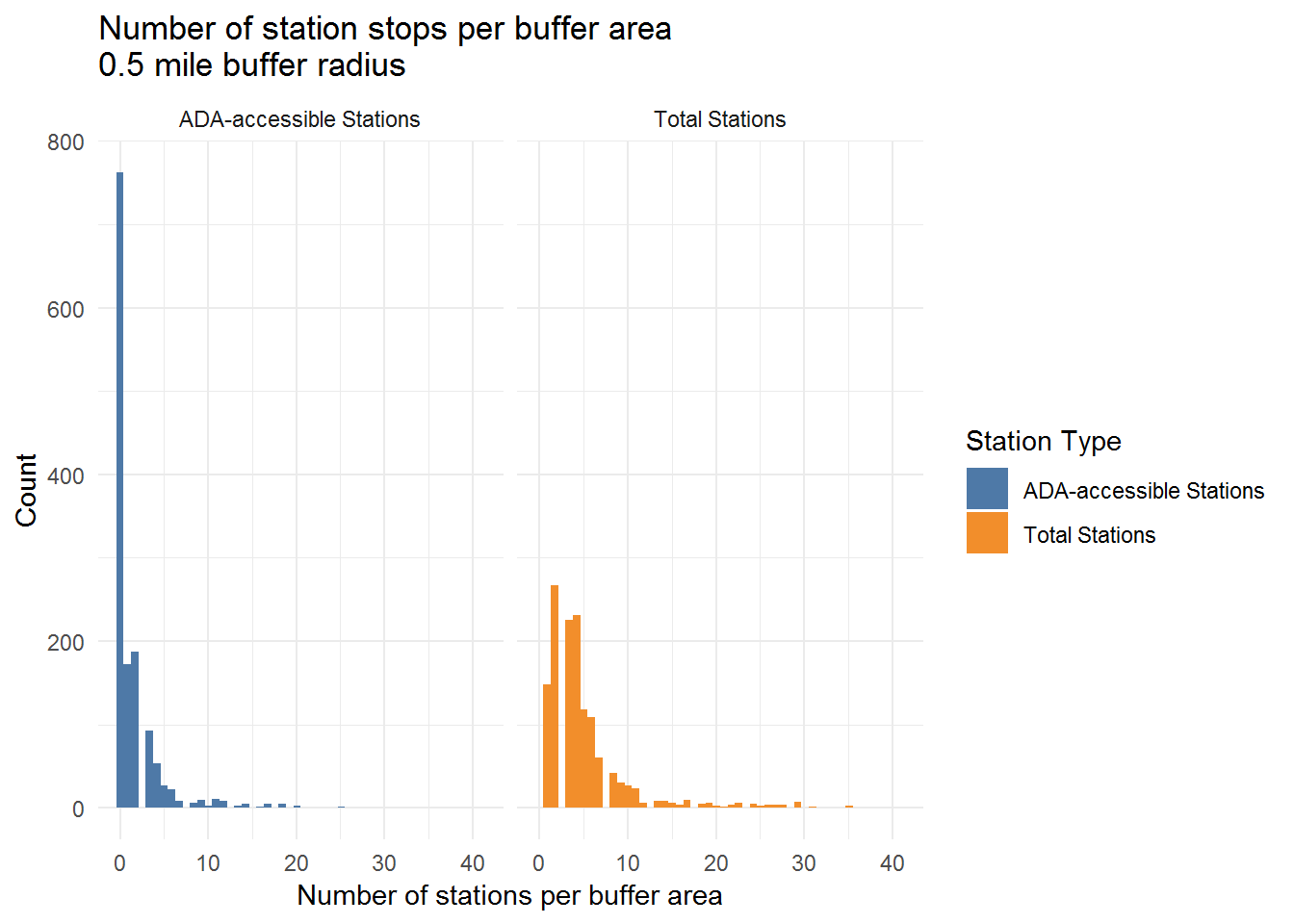

So the cut() function needs to be used again to break up the count data into groups.

nyc.4boro.buff.join %>% 
  mutate(tot_fact = cut(tot_stat, quantile(tot_stat, na.rm = TRUE), include.lowest = TRUE)) %>% 
  ggplot() +
  geom_sf(aes(fill = tot_fact), color = "black") +
  scale_fill_viridis_d(option = "D", name = "Station Count Quantiles", na.value = "gray50") +
  theme(axis.text.x = element_blank(), axis.text.y = element_blank()) +
  ggtitle("Number of subway station stops within tract buffer\nAll stations")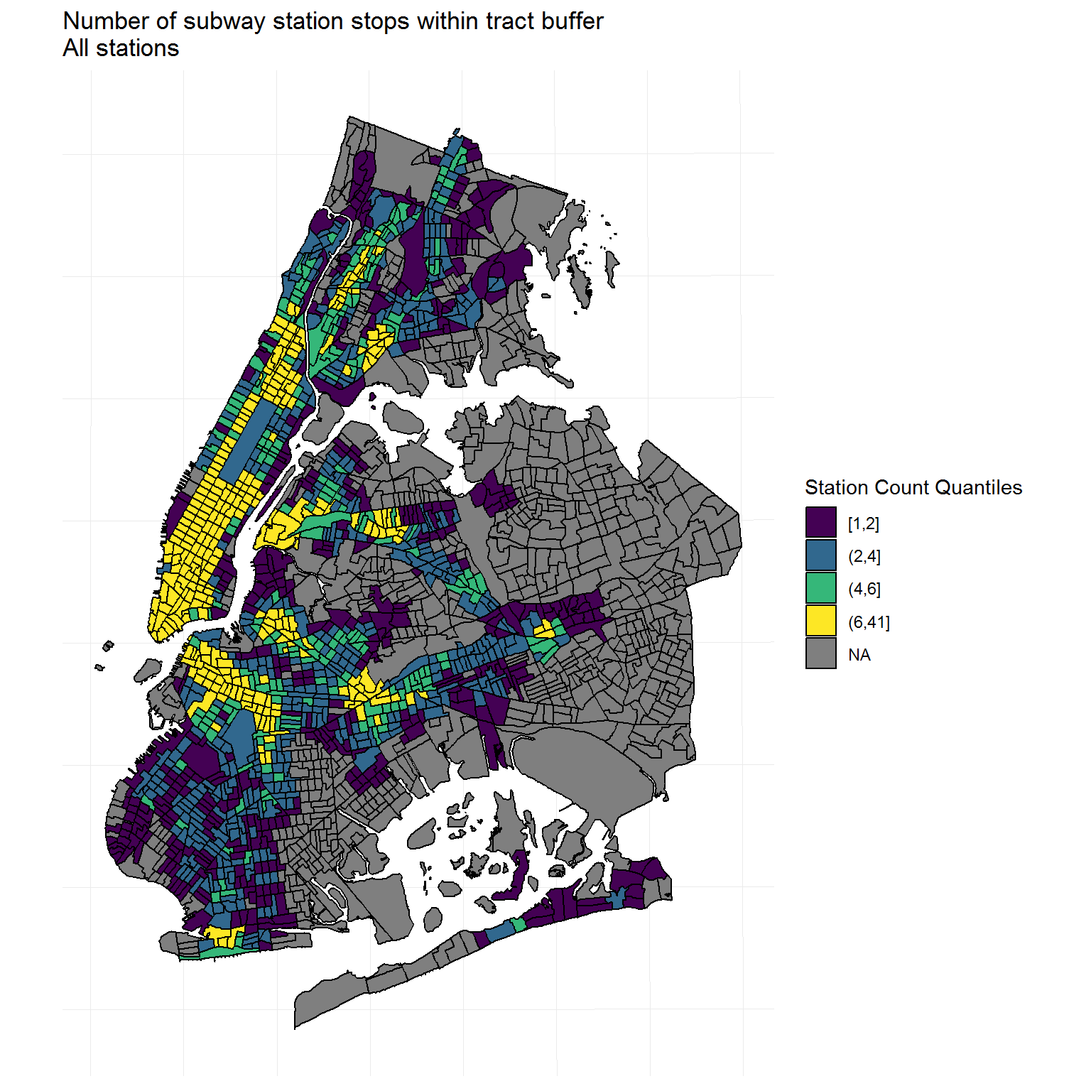

The ADA-accessible station stop per buffer count does not have unique quantiles, but I can instead set the breaks to match the map above so that the scale will be somewhat comparable (except for the maximum).

nyc.4boro.buff.join %>% 
  mutate(
    ada_stat = ifelse(ada_stat == 0, NA, ada_stat),
    # have to give own breaks because quintiles are not unique - 50% of data between 1 and 2
    ada_fact = cut(ada_stat, breaks = c(1, 2, 4, 6, 33), include.lowest = TRUE)
    ) %>% 
  ggplot() +
  geom_sf(aes(fill = ada_fact), color = "black") +
  scale_fill_viridis_d(option = "D", name = "Station Count Breaks", na.value = "gray50") +
  theme(axis.text.x = element_blank(), axis.text.y = element_blank()) +
  ggtitle("Number of subway station stops within tract buffer\nADA-accessible only")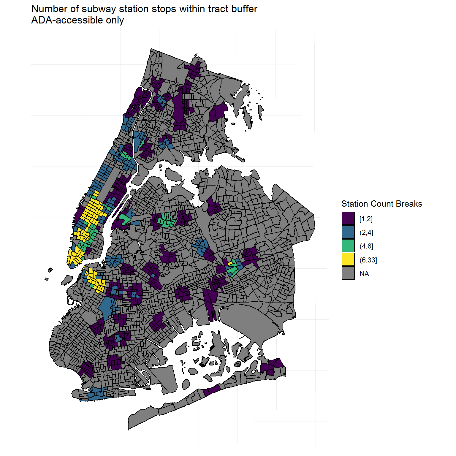

These two maps show that most of the Manhattan census tracts are within a half mile radius of 6 or more subway train route stops (isn’t that a mouthful). Simply speaking, there’s a lot of trains that stop all over Manhattan. This isn’t really a surprise since Manhattan is a transportation hub where all trains, except for the G, either cross from one borough to another or start/end in. That’s just how the city is laid out. Manhattan also has large areas of high ADA subway accessibility, especially south of Central Park. The other boroughs, in comparison, have what can be described as islands of accessibility, serviced by only 1 or 2 subway routes.

As an aside, in the neighborhood shapefile, the parks and airports were grouped into one neighborhood per borough, so I had blocked them out from the maps. In the census tract shapefile, each park and airport is its own tract, which makes the station stop count for these areas more meaningful and so they were left in.

Here’s the interactive version of the total station count map to make the data easier to explore, including which neighborhood the census tracts belong in.

nyc.4boro.buff.join %>% 
  select(boroname, boroct2010, ntacode:ntaname, tot_stat:ada_percent) %>% 
  mutate(`Total Station Count` = cut(tot_stat, quantile(tot_stat, na.rm = TRUE), include.lowest = TRUE)) %>% 
  mapview(zcol = "Total Station Count")

The Queens and Bronx tracts look, by eye, to be larger than tracts in Manhattan and Brooklyn. Also, Queens seems to have less subway coverage than the other boroughs. Let’s calculate some rough estimates of subway coverage and compare what percentage of each borough’s tracts are within half a mile of a subway station.

nyc.4boro.buff.join %>% 
  st_set_geometry(NULL) %>% 
  # remove parks and airports 
  filter(!(str_detect(ntaname, "park") | str_detect(ntaname, "Airport"))) %>% 
  # 1 if tract has subway access within half a mile, 0 otherwise:
  mutate(has_stat = ifelse(!(is.na(tot_stat)), 1, 0)) %>% 
  group_by(boroname) %>% 
  summarize(
    # avg tract area in miles:
    mean_tract_area = round(mean(shape_area) / 5280 ** 2, 3),
    # total borough area miles:
    tot_area = round(sum(shape_area) / 5280 ** 2, 3),
    # total number of tracts per borough:
    tot_tract = n(),
    # number of tracts with subway access:
    tract_w_sub = sum(has_stat),
    # percent of tracts with subway access:
    per_tract_w_sub_access = round(tract_w_sub / tot_tract * 100, 2)
  ) %>% 
  arrange(desc(per_tract_w_sub_access))

# A tibble: 4 x 6
  boroname  mean_tract_area tot_area tot_tract tract_w_sub per_tract_w_sub~
  <fct>               <dbl>    <dbl>     <int>       <dbl>            <dbl>
1 Manhattan           0.07      19.6       281         273             97.2
2 Brooklyn            0.082     61.3       750         587             78.3
3 Bronx               0.104     34.6       332         239             72.0
4 Queens              0.138     89.9       651         279             42.9

These quick calculations confirm the intuition that Manhattan has a lot of subway coverage and Queens has relatively little compared to the other boroughs. But take this with a grain of salt, since Queens and Bronx census tracts are generally larger than those in Manhattan and Brooklyn, and Queens is just huge in terms of area compared to the other boroughs. Perhaps, this result is best used to highlight how surprisingly few of the subway stations in southern Brooklyn are ADA-accessible, even though the borough itself has relatively high subway coverage.

Now, to compare this analysis to the “By Neighborhood” approach, let’s similarly group the tracts and map the results.

nyc.4boro.buff.join <- nyc.4boro.buff.join %>% 
    mutate(
    tract_group = case_when(
      str_detect(ntaname, "park") ~ "Park",
      str_detect(ntaname, "Airport") ~ "Airport",
      !(str_detect(ntaname, "park") | str_detect(ntaname, "Airport")) & is.na(tot_stat) ~ "No stations",
      !(str_detect(ntaname, "park") | str_detect(ntaname, "Airport")) & tot_stat > 0 & ada_stat < 1 ~ "No accessible stations",
      !(str_detect(ntaname, "park") | str_detect(ntaname, "Airport")) & tot_stat > 0 & ada_stat > 0 ~ "At least one accessible station",
      TRUE ~ "Don't know"
      )
    )
nyc.4boro.buff.join %>% 
  ggplot() +
  geom_sf(aes(fill = tract_group)) +
  scale_fill_manual(values = c("grey30", "#0072B2", "#E69F00", "#999999", "#bae4b3"), name = "Tract Type") +
  # overlay neighborhoods in black outline:
  geom_sf(data = nyc.neigh.4boro, color = "black", fill = NA)  +
  theme(axis.text.x = element_blank(), axis.text.y = element_blank()) +
  ggtitle("NYC census tract accessibility\n0.5 mile buffer radius")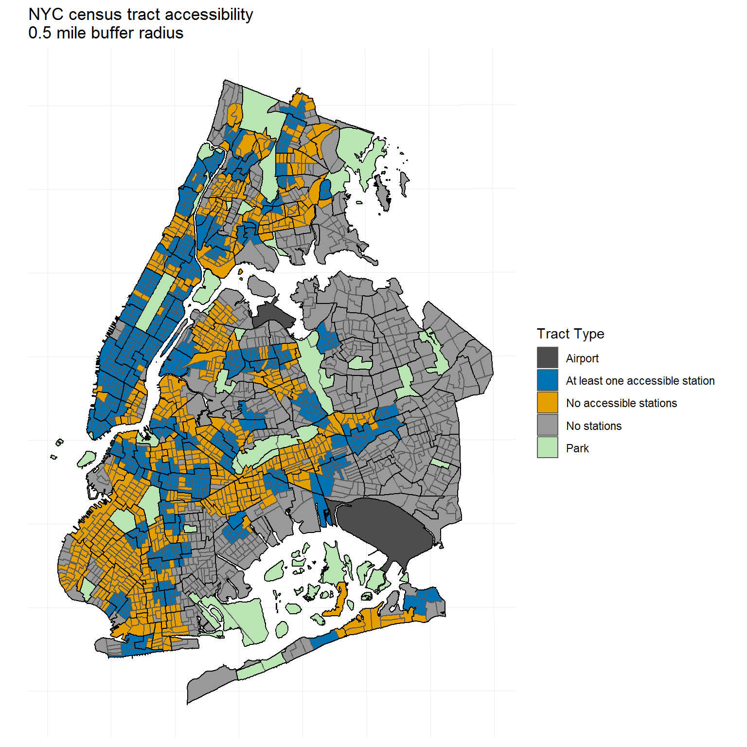

As a reminder, here’s the neighborhoods-based map again, without the subway overlay.

neigh.map.count.prep %>% 
  ggplot() +
  geom_sf(aes(fill = neigh_group), color = "black") +
  scale_fill_manual(values = c("grey30", "#0072B2", "#E69F00", "#999999", "#bae4b3"), name = "Neighborhood Type") + 
  theme(axis.text.x = element_blank(), axis.text.y = element_blank()) +
  ggtitle("Neighborhoods with no accessible subway station")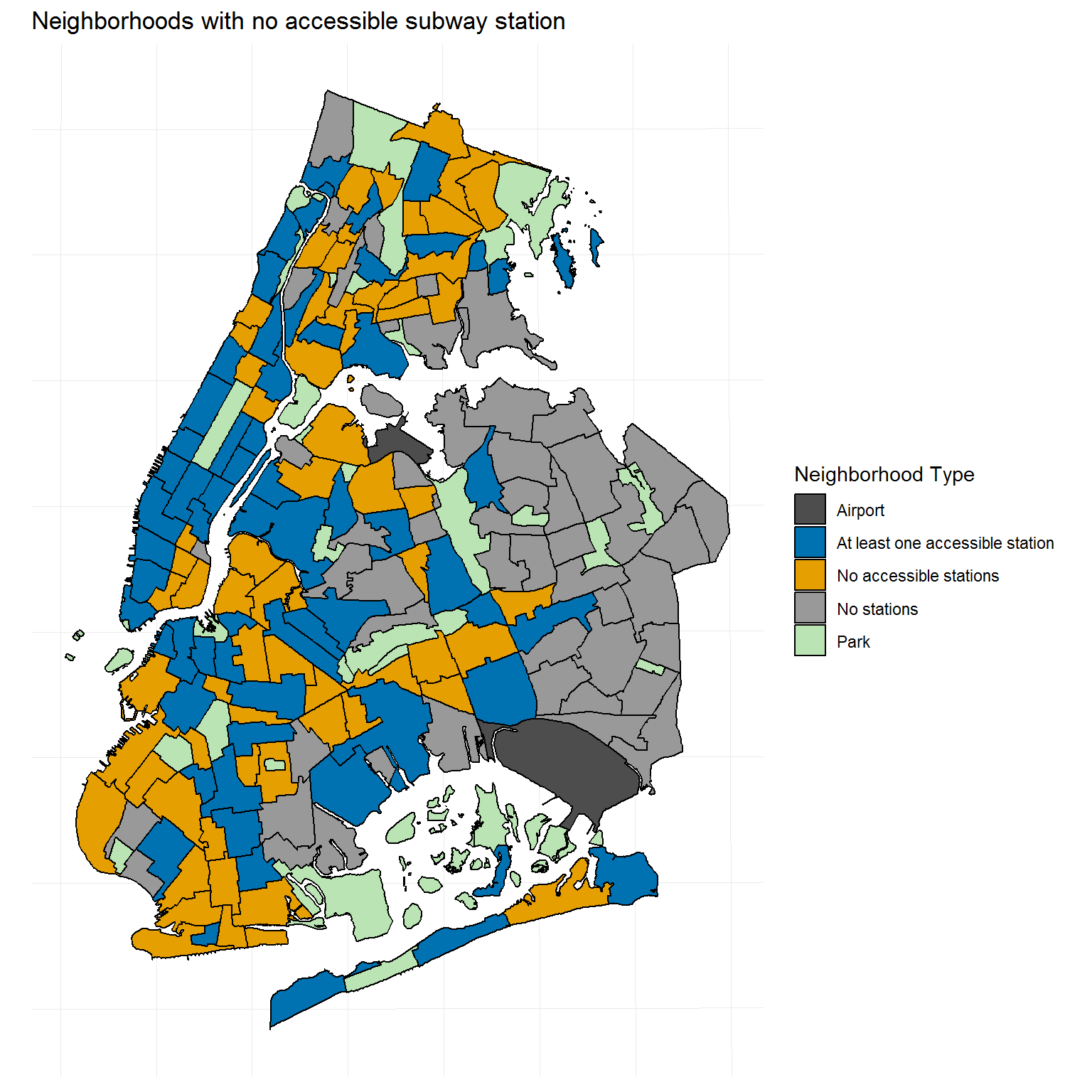

While one can squint at the two maps and try to pick out the differences, it would be easier to compare the two by assigning each tract its accessibility group “by neighborhood” (each tract is within a neighborhood, so it simply inherits this assignment from the neighborhood that its in) and “by tract.”

nyc.4boro.buff.join %>% 
  inner_join(neigh.map.count.prep %>% st_set_geometry(NULL), by = "ntaname") %>% 
  {table(.$tract_group, .$neigh_group, dnn = c("by tract method", "by neighborhood method"))}

                                 by neighborhood method
by tract method                   Airport At least one accessible station
  Airport                               2                               0
  At least one accessible station       0                             448
  No accessible stations                0                             221
  No stations                           0                             111
  Park                                  0                               0
                                 by neighborhood method
by tract method                   No accessible stations No stations Park
  Airport                                              0           0    0
  At least one accessible station                    154          21    0
  No accessible stations                             485          49    0
  No stations                                        104         421    0
  Park                                                 0           0   39

It looks like the “No station” assignments largely match between the two methods, but there are more mismatches in the “At least one accessible station” and “No accessible stations” categories.

Since there are 9 combinations of categories besides Park and Airport, it would probably look like a mess on a map, but it is possible to visualize which tracts are the same, versus those that got a different assignment under the census tract buffer analysis.

nyc.4boro.buff.join %>% 
  inner_join(neigh.map.count.prep %>% st_set_geometry(NULL), by = "ntaname") %>% 
  mutate(
    group_diff = case_when(
      tract_group == "Park" ~ "Park",
      tract_group == "Airport" ~ "Airport",
      tract_group == neigh_group ~ "Same",
      TRUE ~ "Different"
    )
  ) %>% 
  ggplot() +
  geom_sf(aes(fill = group_diff)) +
  scale_fill_manual(values = c("grey30", "#d95f02", "#bae4b3", "#7570b3"), name = "Tract Type") +
  geom_sf(data = nyc.neigh.4boro, color = "black", fill = NA)  +
  theme(axis.text.x = element_blank(), axis.text.y = element_blank()) +
  ggtitle("Group assignment differences\nNeighborhood vs tract buffer analysis")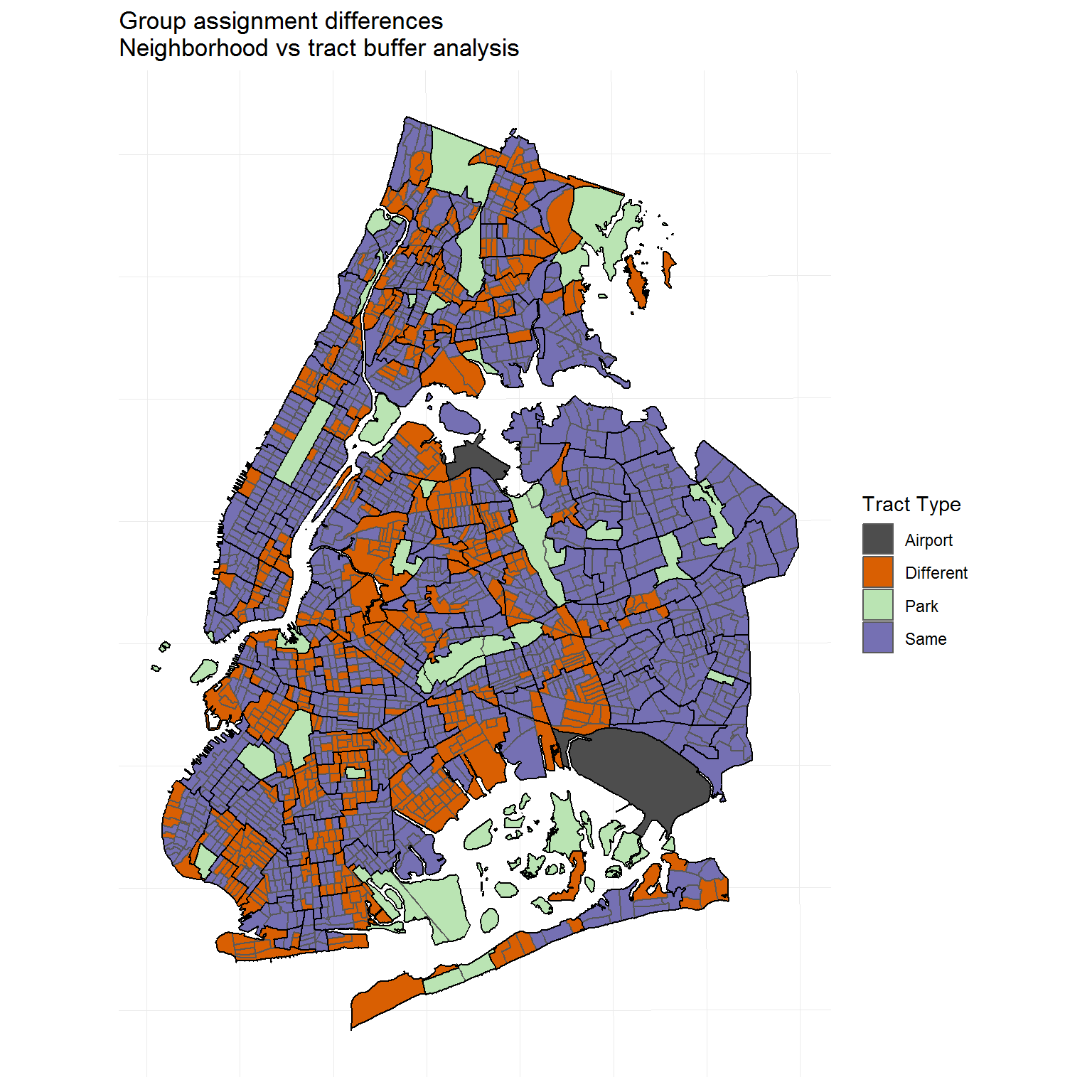

That’s a lot of orange!

And let’s compare specifically areas of accessibility differences:

access.diff <- nyc.4boro.buff.join %>% 
  inner_join(neigh.map.count.prep %>% st_set_geometry(NULL), by = "ntaname") %>% 
  mutate(
    access_diff = case_when(
      # parks and airports are the same in both
      tract_group == "Park" ~ "Park",
      tract_group == "Airport" ~ "Airport",
      # both methods accessible
      tract_group == "At least one accessible station" & neigh_group == "At least one accessible station" ~ "Both Accessible",
      # different assignments
      tract_group != "At least one accessible station" & neigh_group == "At least one accessible station" ~ "Neigh Access / Tract No",
      tract_group == "At least one accessible station" & neigh_group != "At least one accessible station" ~ "Tract Access / Neigh No",
      # Other is either no subway station at all or no accessible station for both methods
      TRUE ~ "Other"
    )
  ) 
table(access.diff$access_diff)

                Airport         Both Accessible Neigh Access / Tract No 
                      2                     448                     332 
                  Other                    Park Tract Access / Neigh No 
                   1059                      39                     175 

access.diff %>% 
  ggplot() +
  geom_sf(aes(fill = access_diff)) +
  scale_fill_manual(values = c("grey30", "#7570b3", "#d95f02", "#999999", "#bae4b3", "#e7298a"), name = "Tract Type") +
  geom_sf(data = nyc.neigh.4boro, color = "black", fill = NA)  +
  theme(axis.text.x = element_blank(), axis.text.y = element_blank()) +
  ggtitle("ADA-accessibility difference\nNeighborhood vs tract buffer analysis")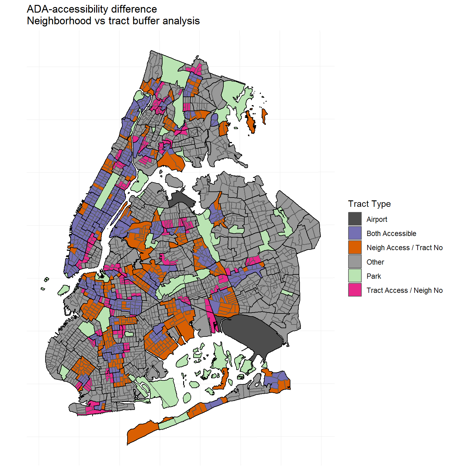

Overall, the “By Neighborhood” approach was more forgiving in assessing accessibility, although some areas were found to be accessible by the tract buffer method and not the neighborhoods approach.

Last, but not least, here is a map of the census tracts by percentage of subway station stop accessibility. Tracts with no accessible stations within their buffer area are once again in orange, and the percent accessibility value is binned into 20% intervals.

nyc.tract.notada <- nyc.4boro.buff.join %>% 
  filter(ada_stat == 0)
nyc.4boro.buff.join <- nyc.4boro.buff.join %>% 
  mutate(ada_percent = ifelse(ada_percent == 0, NA, ada_percent))
nyc.4boro.buff.join$ada_per_breaks <- as.character(cut(nyc.4boro.buff.join$ada_percent, breaks = seq(0, 100, 20)))
nyc.4boro.buff.join %>% 
  mutate(
    ada_per_breaks = ifelse(
      ntacode %in% nyc.parks.air.sf$ntacode, "Park / Airport",
      ifelse(
        boroct2010 %in% nyc.tract.notada$boroct2010, "No accessible stations", ada_per_breaks
        )
      )
    ) %>% 
  ggplot() +
  geom_sf(aes(fill = ada_per_breaks)) +
  scale_fill_manual(values = c("#c7e9b4", "#7fcdbb", "#41b6c4", "#2c7fb8", "#253494", "#b8652c", "grey30"), na.value = "gray50", name = "Percent ADA") +
  theme(axis.text.x = element_blank(), axis.text.y = element_blank()) +
  ggtitle("Percent of ADA-accessible subway station stops\nPer 0.5mi radius buffer")

It is interesting that the dark blue areas in the outer boroughs correspond with the final subway route stops. Perhaps what stands out more are the last stops that are not accessible, particularly the 95th St Bay Ridge R stop in Brooklyn (marked with a large white circle below). The final route stations that are noticeably not accessible are:

• White Circle - 95st Bay Ridge / R train / Brooklyn
• White Square - New Lots Ave / 3 train / Brooklyn
• Yellow Circle - Eastchester-Dyre Ave / 5 train / Bronx
• Yellow Square - Woodlawn / 4 train / Bronx

nyc.4boro.buff.join %>% 
  mutate(ada_per_breaks = ifelse(ntacode %in% nyc.parks.air.sf$ntacode, "Park / Airport",ifelse(boroct2010 %in% nyc.tract.notada$boroct2010, "No accessible stations", ada_per_breaks))) %>% 
  ggplot() +
  geom_sf(aes(fill = ada_per_breaks)) +
  scale_fill_manual(values = c("#c7e9b4", "#7fcdbb", "#41b6c4", "#2c7fb8", "#253494", "#b8652c", "grey30"), na.value = "gray50", name = "Percent ADA") +
  geom_sf(data = sub.sf.nyc.crs, color = "grey90", fill = "black", size = 2, pch = 21) +
  # last R stop in Brooklyn
  geom_sf(data = sub.sf.nyc.crs %>% filter(stat_name == "bmt_4 avenue_95th st"), color = "white", size = 3) +
  # last 5 stop in Bronx
  geom_sf(data = sub.sf.nyc.crs %>% filter(stat_name == "irt_dyre av_eastchester-dyre av"), color = "yellow", size = 3) +
  # last 3 stop in Brooklyn
  geom_sf(data = sub.sf.nyc.crs %>% filter(stat_name == "irt_new lots_new lots av"), color = "white", size = 3, shape = 15) +
  # last 4 stop in Bronx
  geom_sf(data = sub.sf.nyc.crs %>% filter(stat_name == "irt_jerome_woodlawn"), color = "yellow", size = 3, shape = 15) +
  theme(axis.text.x = element_blank(), axis.text.y = element_blank()) +
  ggtitle("Percent of ADA-accessible subway station stops\nPer 0.5mi radius buffer")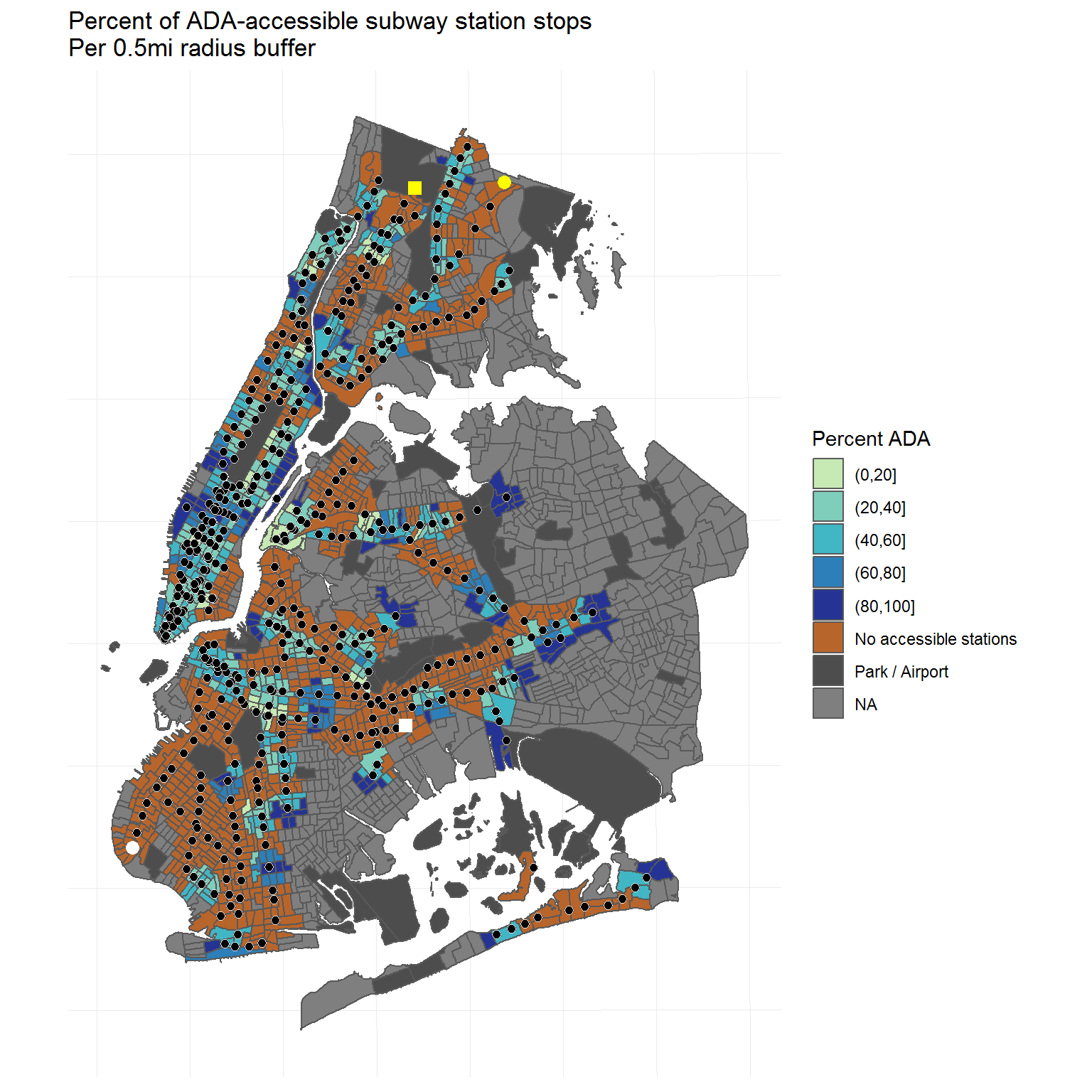

These stations might be good first choices for ADA-accessibility conversion.